<?xml version="1.0" encoding="utf-8"?><feed xmlns="http://www.w3.org/2005/Atom" ><generator uri="https://jekyllrb.com/" version="4.4.1">Jekyll</generator><link href="/feed.xml" rel="self" type="application/atom+xml" /><link href="/" rel="alternate" type="text/html" /><updated>2026-05-14T16:44:17+00:00</updated><id>/feed.xml</id><title type="html">Way Lab</title><subtitle>Biomedical data science</subtitle><entry><title type="html">coSMicQC: A step toward quality control and improvement of morphology profiles</title><link href="/2024/12/20/cosmicqc.html" rel="alternate" type="text/html" title="coSMicQC: A step toward quality control and improvement of morphology profiles" /><published>2024-12-20T00:00:00+00:00</published><updated>2024-12-20T00:00:00+00:00</updated><id>/2024/12/20/cosmicqc</id><content type="html" xml:base="/2024/12/20/cosmicqc.html"><![CDATA[<h1 id="lets-tour-the-single-cell-morphological-galaxy-with-cosmicqc">Let’s tour the single-cell morphological galaxy with coSMicQC!</h1>

<p>Hi everyone! 🤩</p>

<p>I’m back with another blog post! 
This time, I want to share something I’ve become very excited and passionate about:</p>

<p>✨ <em>Quality control of single-cell morphology profiles</em> ✨</p>

<p>I will go over what is quality control for morphology profiles, existing work on this topic, the software (coSMicQC) that we have developed to help in this area, and where we hope to go from here.</p>

<h2 id="contents">Contents</h2>

<ol>
  <li>📋 <a href="#defining-quality-control-of-single-cell-morphology-profiles">What is quality control for single-cell morphology profiles?</a></li>
  <li>📉 <a href="#what-quality-control-methods-currently-exist">What are the current methods for addressing this topic?</a></li>
  <li>🌌 <a href="#introduction-to-cosmicqc">Introduction to coSMicQC</a></li>
  <li>🎯 <a href="#example-of-cosmicqc-impact">Example of coSMicQC’s impact</a></li>
  <li>🚀 <a href="#whats-next">Where do we go from here?</a></li>
</ol>

<h2 id="defining-quality-control-of-single-cell-morphology-profiles">Defining quality control of single cell morphology profiles</h2>

<blockquote>
  <p><strong>Quality Control (QC)</strong><br />
The process of validating and enforcing a specific standard across all products.</p>
</blockquote>

<blockquote>
  <p><strong>Single-cell morphology profiles</strong><br />
Features (e.g., area, texture, intensity, etc.) extracted from images of cells. 
Traditionally, profiles are formatted in a dataframe where each row is single-cell, and columns are either metadata or feature extracted from a specific segmented part of a cell (e.g., nucleus, whole cell, or cytoplasm).</p>
</blockquote>

<p>Putting these two definitions together, single-cell quality control is the process of enforcing a standard quality based on single-cell morphology features, which we measure based on segmentation.</p>

<h3 id="background-on-image-based-profiling">Background on image-based profiling</h3>

<p>
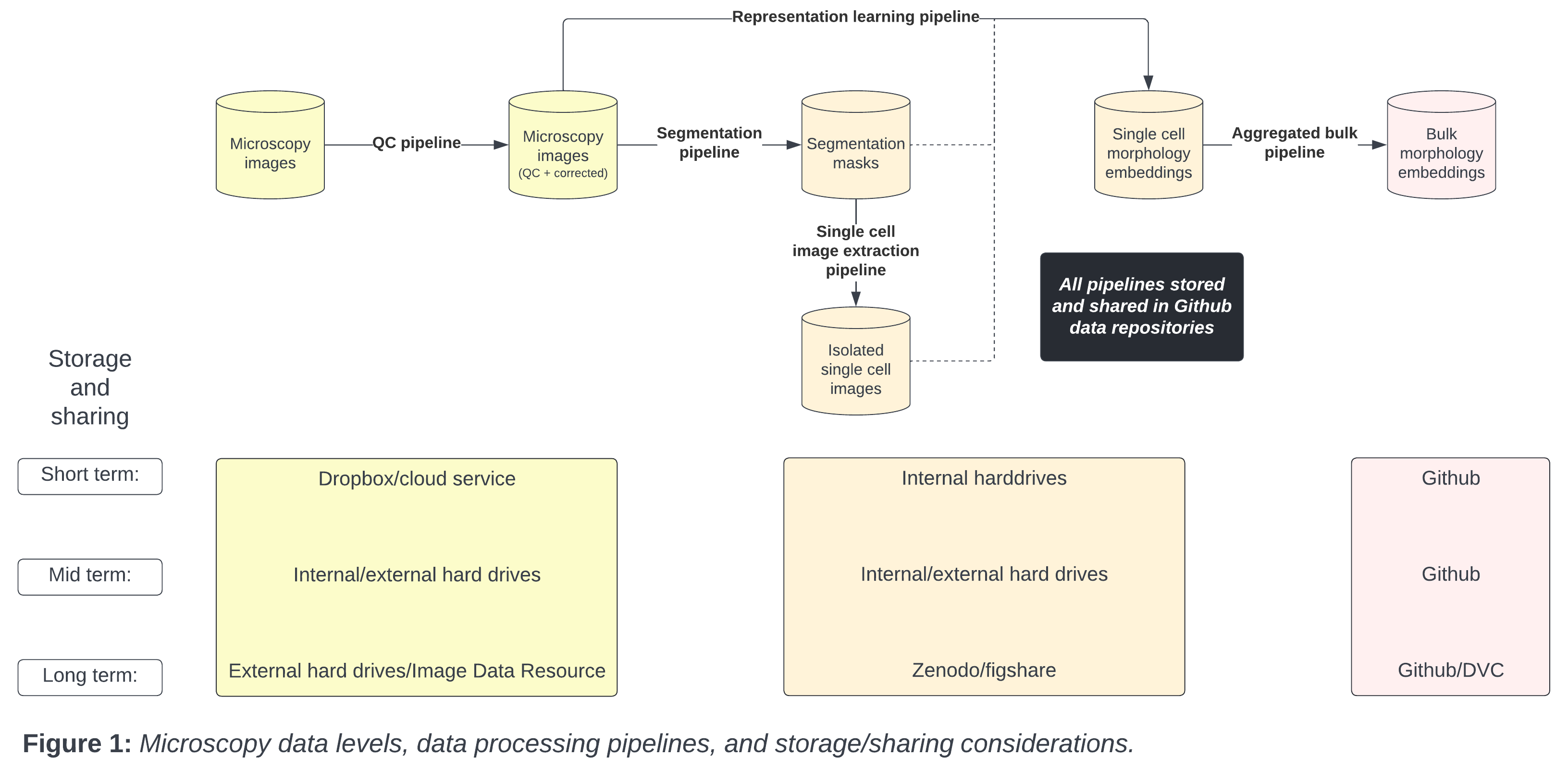
If you are unfamiliar to the standard process of image-based profiling, there are typically 3 main steps after collecting raw images:
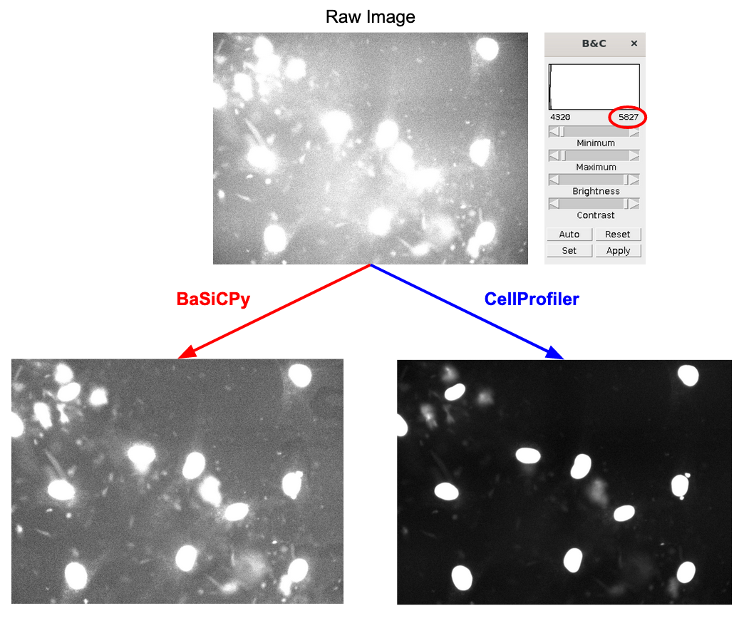
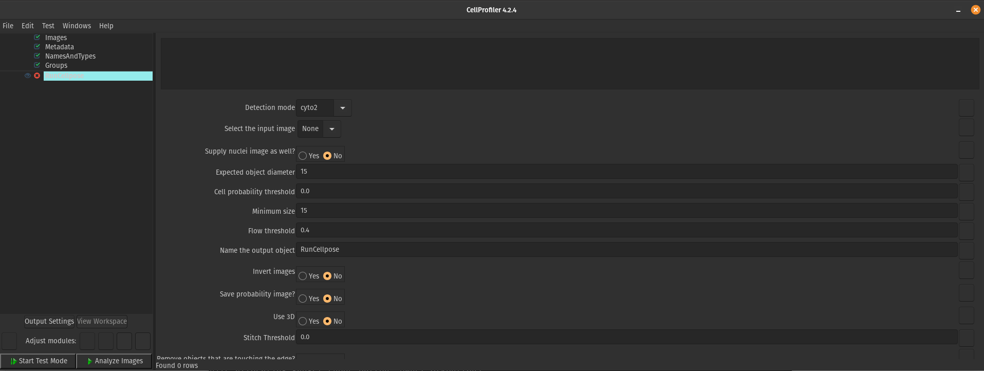
</p>

<figure class="figure">
  <a class="figure_image" style="width: 100%;">
    <img src="/images/blog/cosmicqc/simple_image_based_profiling.png" alt="Simple workflow for image-based profiling including intermediate steps for CellProfiler, CytoTable, and pycytominer." title="Simple workflow for image-based profiling including intermediate steps for CellProfiler, CytoTable, and pycytominer." style="width: 100%;" loading="lazy" />
  </a><figcaption class="figure_caption">Simple workflow for image-based profiling including intermediate steps for CellProfiler, CytoTable, and pycytominer.
</figcaption></figure>

<p>The software called <a href="https://cellprofiler.org/">CellProfiler</a> typically extracts morphology features from images. 
There are other feature extraction software (like Molecular Devices IN Carta), but we will be focusing on CellProfiler in this blog post. 
Researchers use CellProfiler to perform the first steps of a standard image-based analysis workflow, such as illumination correction, segmentation (traditionally of nuclei, cells, and cytoplasm), and feature extraction.
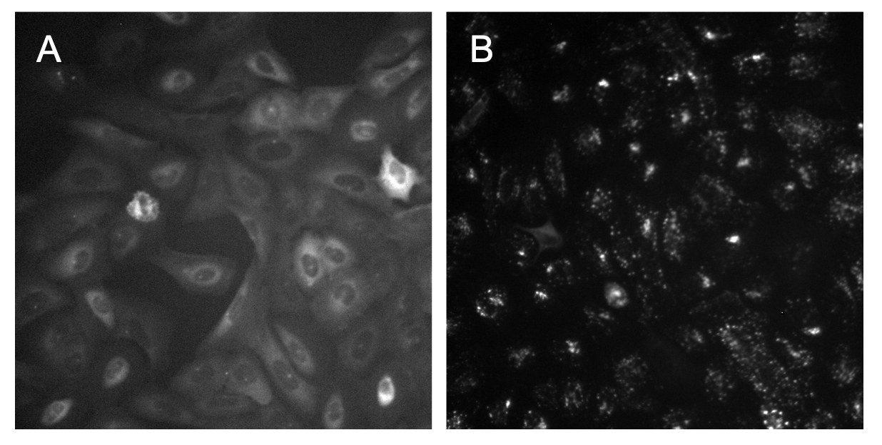
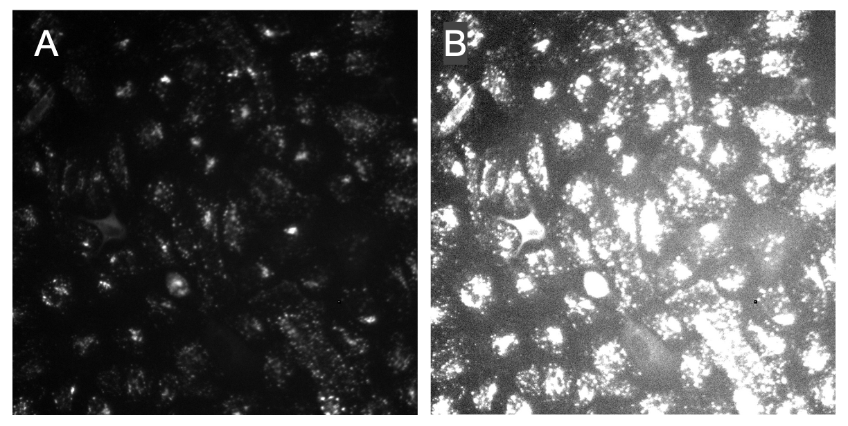
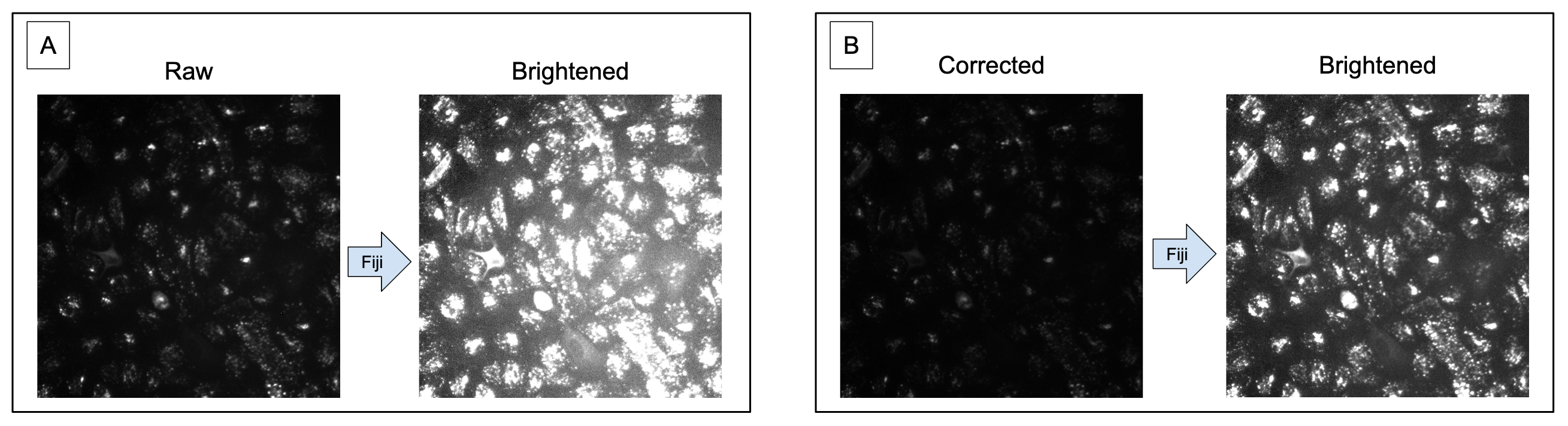
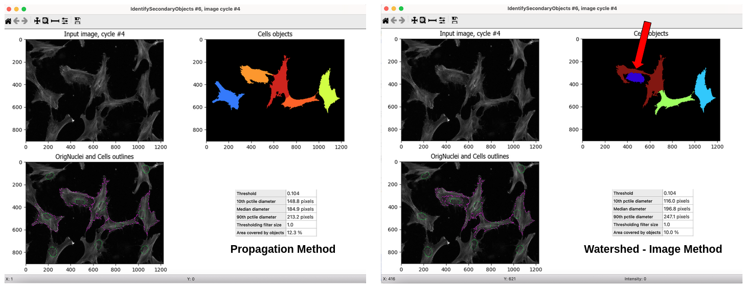
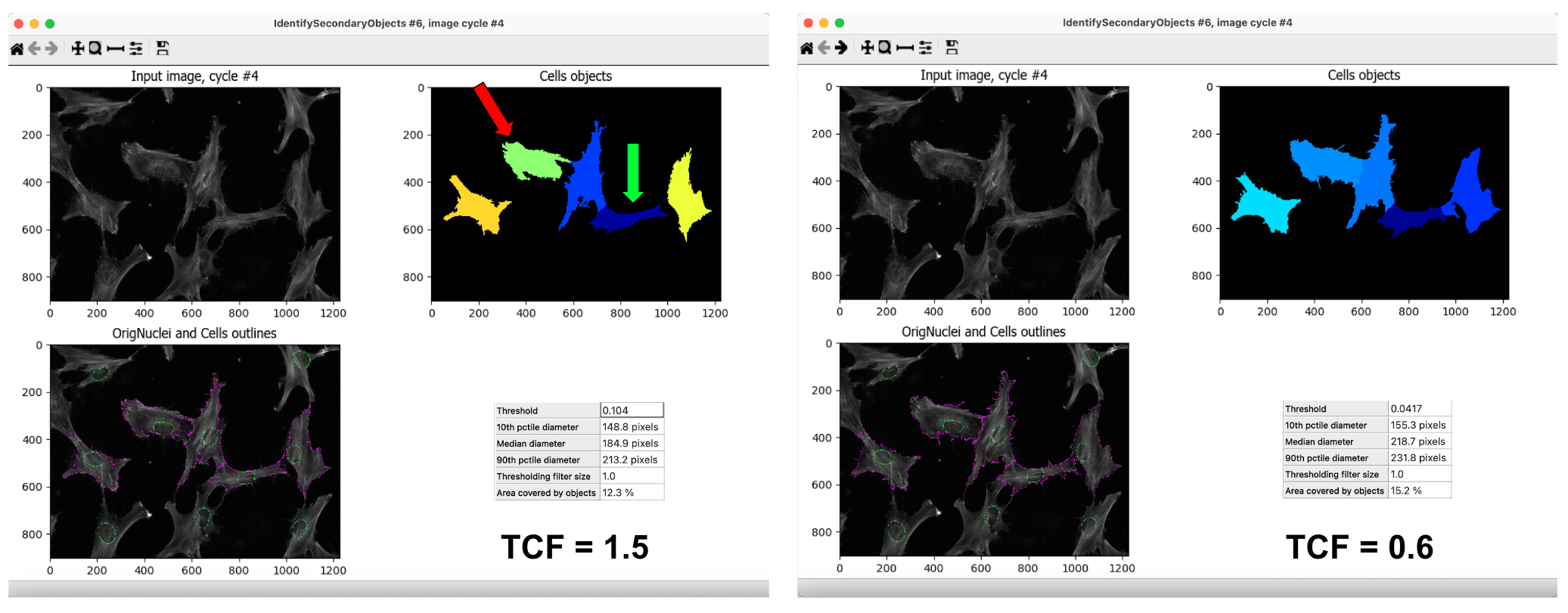
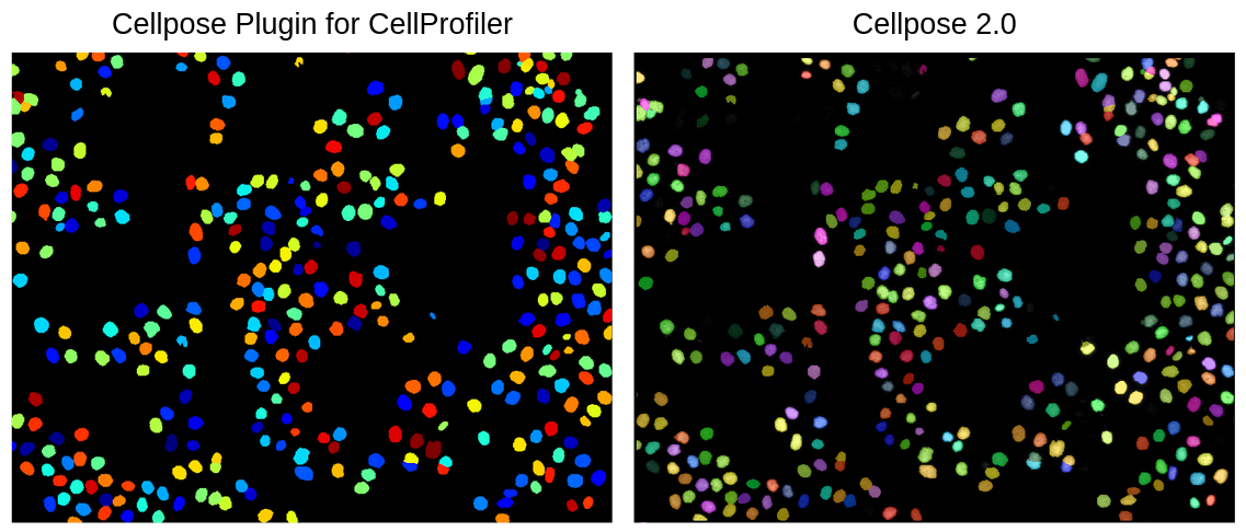
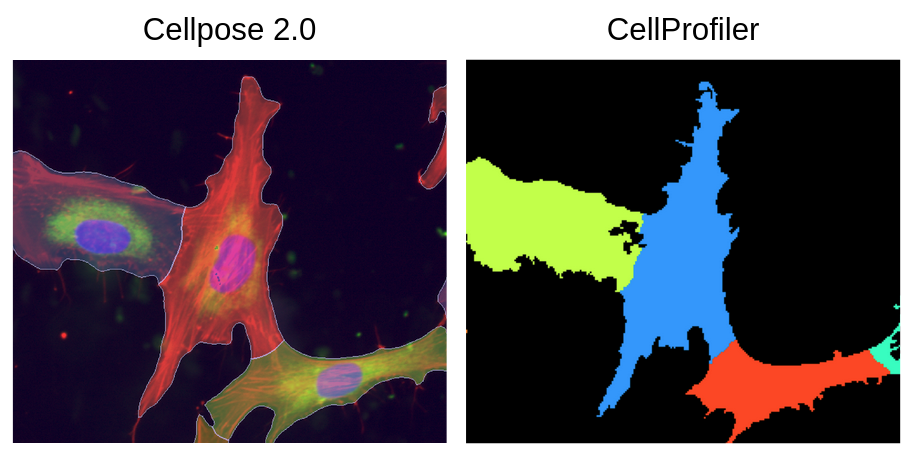
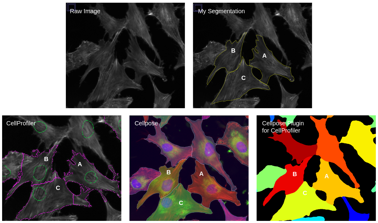
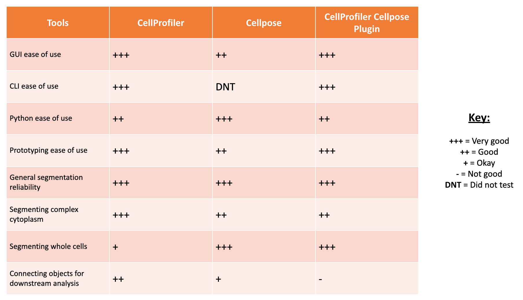
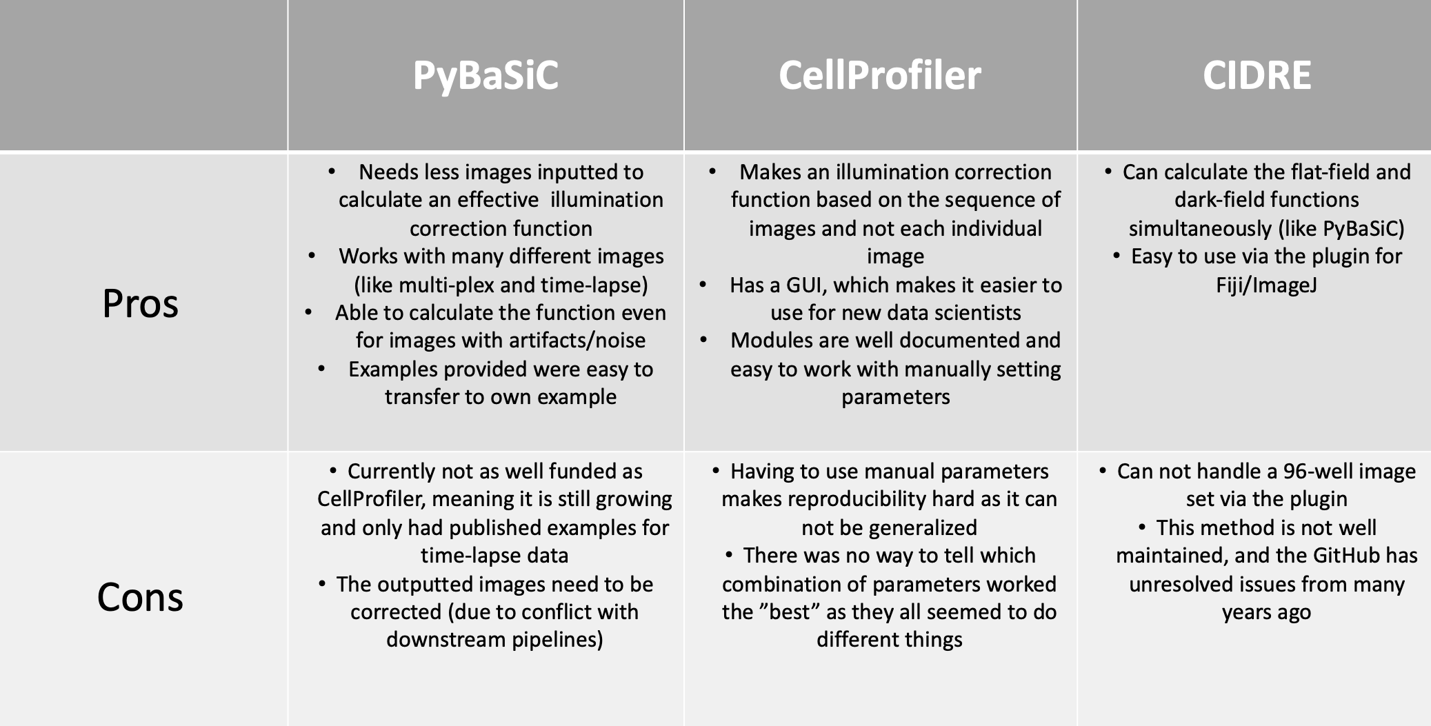
</p>

<p><strong>PLUG TIME!</strong>
If you aren’t familiar with illumination correction (IC) or want to learn more, feel free to read the two blog posts on the topic, “<a href="https://www.waysciencelab.com/2022/08/09/illumcorrect.html">Illumination Correction Made Easier</a>” and “<a href="https://www.waysciencelab.com/2023/08/07/illumsteps.html">Steps for Performing Illumination Correction in Microscopy Images</a>”. 
I also wrote a blog post regarding the pros and cons of two segmentation methods if you are interested called “<a href="https://www.waysciencelab.com/2022/11/01/segmentation.html">Segmentation Software Usability and Performance: Part I</a>”.
<strong>OKAY, PLUG TIME OVER!</strong></p>

<p>The next step in the workflow is <a href="https://cytomining.github.io/CytoTable/">CytoTable</a>, which reformats the output from CellProfiler (and other feature extraction software), to create a standardized parquet file where each row is a single-cell and the columns are the combined features per cell.</p>

<p>Lastly, researchers preprocess the standardized output before performing analysis and machine learning. 
Researchers will then aggregate single-cell features to the well-level population, either by taking the median or mean.
This process can be done within a software called, <a href="https://pycytominer.readthedocs.io/en/stable/">pycytominer</a>, which is optimized to process morphological profiles from multiple outputs.</p>

<p>Aggregation removes the heterogeneity of the population and reduces noise.
But, this “reduction of noise” is a bit fishy to me. 🐟
If you aggregate a bunch of poorly segmented single-cell profiles, then aggregating will just exacerbate the issue and mis-represent the biology of the population.
This leads me into why I think quality control at the single-cell level for morphology profiles is a necessary step, regardless of if you plan to process your data as bulk (aggregated) or single cells.</p>

<h3 id="why-single-cell-quality-control">Why single-cell quality control?</h3>

<p>Quality control of single-cell profiles is very important to avoid mis-interpretation of the results, and ensure that downstream analysis is picking up biologically relevant information.</p>

<p>Imagine you have an picture of cells and you want to cut out each individual cell.
As you are cutting, your hand could end up slipping or you get distracted, so your individual cell cut-out ends up missing part of the cell.
This is what a segmentation error is. 
These cut-outs with incomplete cells are missing vital and biological information about that cell.
Quality control acts like a checklist, ensuring that each cut-out meets the required standards, such as verifying that no parts of the cell are missing.</p>

<figure class="figure">
  <a class="figure_image" style="width: 100%;">
    <img src="/images/blog/cosmicqc/segmentation_cartoon.png" alt="Simplified representation of single-cell segmentation." title="Simplified representation of single-cell segmentation." style="width: 100%;" loading="lazy" />
  </a><figcaption class="figure_caption">Simplified representation of single-cell segmentation.
</figcaption></figure>

<p>In the Way Lab, we traditionally process single-cell data, so we expect heterogeneity within our samples.
We do not want the heterogeneity influenced by technical factors, like poor segmentations.
So, we want to remove any of these poor segmentation before we perform important pre-processing steps like normalization and feature selection.
If we don’t filter poor segmentations, our data processing will include errors, which will reduce the signal-to-noise ratio.</p>

<p>Therefore, we perform quality control for single-cell morphology profiles after CytoTable but before pycytominer.
But, what methodology exists so that we can perform this task?</p>

<hr />

<h2 id="what-quality-control-methods-currently-exist">What quality control methods currently exist?</h2>

<p>If you are familiar with the RNA-seq world, you will know that the concept of <em>Single-cell quality control</em> itself is not new.
It is a well known process within scRNA-seq pipelines where individual cells are filtered out using a metric(s) that detects if it is likely an artifact or contains noise.
It is such a well-established part of this field that there even is <a href="https://www.scrna-tools.org/">a whole website detected to scRNA tools</a>, where you can filter for specifically <a href="https://www.scrna-tools.org/tools?sort=name&amp;cats=QualityControl">quality control tools</a>.
This provides at least one hundred different options to try! 👀 
This is also an important step in not just single-cell, but also bulk RNA-seq as well, which has existed for over two decades.
scRNA-seq has been around for over a decade, so there has been a lot of time to develop these methods across both technologies.</p>

<p><a href="https://journals.plos.org/plosone/article?id=10.1371/journal.pone.0080999">Cell Painting</a> was first developed in 2013, meaning that image-based profiling and extraction of morphological profiles is a new field, but it still has been around for <a href="https://arxiv.org/abs/2405.02767">over a decade</a>.
However, single-cell quality control for morphology profiling is not nearly as thoroughly developed. 😢</p>

<p>This lack of development could be because of the lack of trust in this method, which is described in the 2017 paper, “<a href="https://www.nature.com/articles/nmeth.4397">Data-analysis strategies for image-based cell profiling</a>”.
Caicedo et al. describes some general methods of cell-level outlier detection, including model-free and model-based.
Their main concern is that this method of quality control can assume homogeneity and remove interesting phenotypes (spoiler, we do run into this issue!).
This is why most labs skip this step.
Honestly, this concern applies to all quality control methods and underscores the importance of striving for continuous improvement.</p>

<p>Currently, you are able to “filter objects” (e.g., segmented organelles like nuclei and cytoplasm) in CellProfiler using morphology measurements in its own module.
You can set limits for what feature measurement is considered good or bad, but without exporting the data and exploring the feature space, you do not know the range of feature measurements for your dataset.
In my opinion, this module is good to have, but it isn’t a solution to single-cell quality control.</p>

<p>I checked to see if there were existing single-cell quality control methods for image-based profiling.
I was only able to find one paper, published in BMC Bioinformatics, called “<a href="https://bmcbioinformatics.biomedcentral.com/articles/10.1186/s12859-020-03603-5">A cell-level quality control workflow for high-throughput image analysis</a>”, and it was published in 2020.
It was an interesting read!</p>

<p>For example, in the background section, Qiu et al. state:</p>

<blockquote>
  <p><em>“To our knowledge, this represents the first QC method and scoring metric that operate at the cell level.”</em></p>
</blockquote>

<p>Since I couldn’t find any other paper that focuses on quality control at the single-cell level published before, I completely agree with their statement, they are definitely the first.</p>

<p>I actually did come across another paper after this one (published in 2022) that cites their work, called “<a href="https://journals.plos.org/plosone/article?id=10.1371/journal.pone.0267280">Image-based cell profiling enhancement via data cleaning methods</a>”
The main highlight in this paper, is that they did attempt cell-level outlier detection.
Specifically, Rezvani et al. used a method called Histogram-Based Outlier Score (HBOS).
They utilized the function from a Python package called <a href="https://github.com/yzhao062/pyod">PyOD</a>, a well-established package dedicated to anomaly detection.
Unfortunately, this paper does not include any link to reproducible code for how they used this method to detect outliers with CellProfiler features.
But, they made a very promising statement:</p>

<blockquote>
  <p><em>“It turns out that the cell outlier detection is a more effective method in improving the overall profile quality, while regress-out mainly improves the very top connections.”</em></p>
</blockquote>

<p>Given this claim, we can use this to further fuel the push towards improving single cell quality control.
Unfortunately, this means there are only two papers that are performing this process, so we still have a ways to go. ⏰</p>

<p>But, let’s get back to the first attempt at single cell quality control (Qiu et al. 2020), shall we?</p>

<p>To summarize the paper, they present a cell-level quality control workflow which uses machine learning to detect artifacts within images.
They utilized CellProfiler to segment single cells and extract features from both the cells and whole images.
They wanted to group images based on their phenotype, so they utilized CellProfiler features (like <code class="language-plaintext highlighter-rouge">PowerLogLogSlope</code>, <code class="language-plaintext highlighter-rouge">FocusScore</code>, <code class="language-plaintext highlighter-rouge">MeanIntensity</code>, <code class="language-plaintext highlighter-rouge">Cell Count</code>, etc.) to detect images that contains artifacts versus no artifacts.
Once images were grouped together, they performed a method using kernel density estimate (KDE) to sample the images into their respective phenotypes.
They then trained an SVM (Support Vector Machine) per phenotype group, to classify regions in images where there are artifacts and where there are cells.</p>

<p>This is only a brief summary, so feel free to read the paper if you want a more in-depth look.</p>

<p>What I really liked about this paper is that it is attempting to preserve images that include artifacts, as these images still contain other cells.
It is different than the current process where whole images are removed that fail QC metrics like blur and over-saturation (traditionally done in CellProfiler).</p>

<p>But, I also have my suspicions about using cells that come from an image with corruption, such as an artifact.
I wonder how much things like an artifact or smudge could be directly impacting the biology the cells. 🤔 
This would be a cool research project, but, in my opinion, I would rather lose cells in an image with an artifact than risk any issues in downstream interpretation of the results that might be due to any impacts the artifacts in the image had.</p>

<p>I have two main concerns from this paper, specifically for it’s generalizability and usability in my own pipelines:</p>

<ol>
  <li>It was not clear to me how this method is filtering out artifacts at the single-cell level. From what I understood from the figures, the SVM is able to detect where there is artifacts and where there are cells, but I didn’t see where in their pipeline that they remove single-cells from the CellProfiler output. This is a big concern for generalizability as it seems like you would need to train SVMs on your data to be able to apply this method but there isn’t a direct link to that output and how they actually filtered cells.</li>
  <li>The code is available via FigShare, but it was a bit hard to parse. Since it is not on GitHub, that also limits the usability since there isn’t an environment or dependencies, and there isn’t a way to create issues and contact the maintainers for assistance. As well, I found that the code was not easy to understand and lacked documentation. I want to make clear, I appreciate that they made the code available and open source which is more than some other papers! My main point is that I don’t think this method is feasible to include in my standard workflow.</li>
</ol>

<p>In conclusion, I want to thank the authors of this paper for their hard work and their important contributions to pushing the field towards developing quality control methodology at the single-cell level for morphology profiles.</p>

<p>After the research I conducted and papers I found, I was determined to pursue working on a new methodology, one that is simple, to filter out poor quality segmentations from single-cell morphology profiles.</p>

<hr />

<h2 id="introduction-to-cosmicqc">Introduction to coSMicQC</h2>

<p>
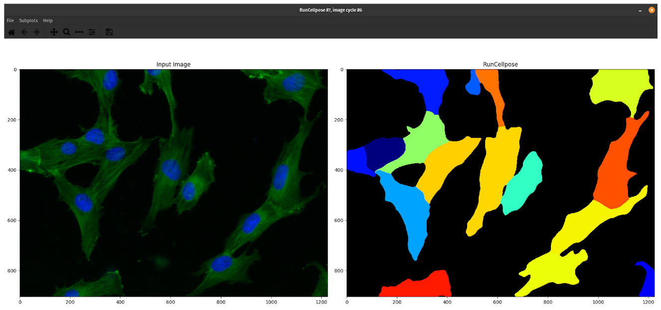
After 2 and half years of being in my position and performing image-based profiling, I have come to realize that I am not perfect (shocking I know! 😱).
No matter how much I try to manually optimize my segmentation parameters in CellProfiler or when using <a href="https://www.cellpose.org/">Cellpose</a> or <a href="https://stardist.net/">Stardist</a>, it will not work for all of the single cells in my datasets.
Now, I am not necessarily saying this is a fault of my own 😉, but segmentation errors are a persistent issue and it is currently a problem that hasn’t been solved to this day.</p>

<p>My point is, you can expect all of your datasets to contain some poorly segmented cells that can be described as technical artifacts.
You can also expect that debris or smudges could also end up being mis-segmented as cells.
When working with single-cell data, we do not want these technical artifacts impacting the interpretation of our results.
Thus, was born this simple idea in my head.</p>

<p>Why not just filter out single cells based on the extracted morphology features?</p>

<p>You wouldn’t need to train any model or perform any other pipeline.
You already have the data in your lap to use, but how you use that data is what is important.
As Caicedo et al. points out, not all features have a normal distribution.
So, we propose a solution to this that focuses on morphology features that are most directly linked to features most correlated to poor segmentation or technical artifacts.</p>

<p>Arriving to the stage is: <em>drum roll please</em> 🥁</p>

<p><a href="https://github.com/WayScience/coSMicQC">coSMicQC</a>, or Single cell Morphology Quality Control!</p>

<figure class="figure">
  <a class="figure_image" style="width: 50%;">
    <img src="/images/blog/cosmicqc/cosmicqc_stage.png" alt="Logo for coSMicQC being shown on a stage, like the star of the show! ⭐️" title="Logo for coSMicQC being shown on a stage, like the star of the show! ⭐️" style="width: 100%;" loading="lazy" />
  </a><figcaption class="figure_caption">Logo for coSMicQC being shown on a stage, like the star of the show! ⭐️
</figcaption></figure>

<p>I want to shout out Dave Bunten (aka @d33bs) here, who has been a major contributor to coSMicQC, which is an open-source software that we are developing with sustainable software development practices! 📣</p>

<p>In summary, coSMicQC uses extracted morphology features directly from CellProfiler, performs normalization of specific features that are most related to detecting poor segmentation, and uses standard deviation to identify single cells that are considered technical outliers.</p>

<p>
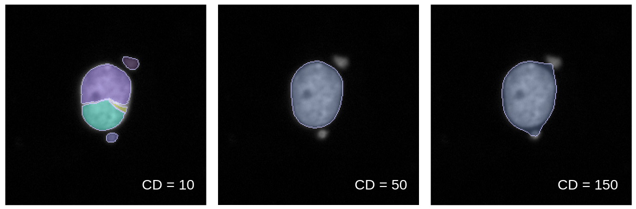
Going into more detail on this new method, it works by first creating conditions.
A condition is a feature or group of features that will capture a specific type of technical artifact.
For example, nuclei area and intensity can work together as a condition to detect large nuclei with high intensity which represents segmentation of clustered/overlapping nuclei.
Your condition will also need how many standard deviations from the mean that you expect these outliers to be located.
If you want to detect cells above a mean, you use a positive value, and vice versa for cells below the mean.</p>

<figure class="figure">
  <a class="figure_image" style="width: 100%;">
    <img src="/images/blog/cosmicqc/area_outlier_example.png" alt="Example of how outliers are detected based on nuclei area in coSMicQC." title="Example of how outliers are detected based on nuclei area in coSMicQC." style="width: 100%;" loading="lazy" />
  </a><figcaption class="figure_caption">Example of how outliers are detected based on nuclei area in coSMicQC.
</figcaption></figure>

<p>You can use the function <code class="language-plaintext highlighter-rouge">find_outliers()</code> to the simple conditions and voila, coSMicQC yields a dataframe with flagged single-cell outliers per condition.
A summary is also outputted, which includes the total number of outliers detected, the percent of the total cells in the data detected as outliers, and the range of the values of the outliers for the features used in the condition.</p>

<p>
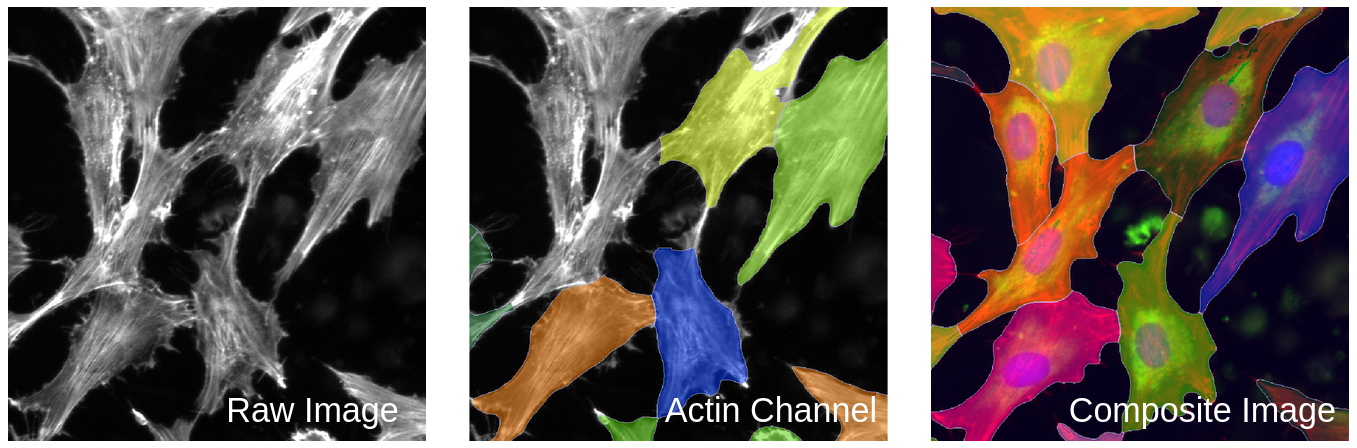
A highlight of coSMicQC is that you are able to visualize single-cell segmentations within the notebook if you provide the original images and exported outlines from CellProfiler, through the use of a novel dataframe format, built on top of <code class="language-plaintext highlighter-rouge">pandas</code>, that we call <a href="https://github.com/WayScience/CytoDataFrame">CytoDataFrame</a>.
This open-source formatter is also developed by Dave Bunten! 📣
This makes it more streamlined to assess if your conditions are working without having to go outside of the notebook and jump to your handy file manager, Fiji, or CellProfiler to see what the segmented cells look like.
This feature is still being developed as we find more datasets with varying conditions for image file structure.</p>

<p>By detecting technical outliers with coSMicQC, further downstream processes should yield higher quality results.
We have been able to test this hypothesis using one of our projects, and further prove that there is merit to pursing single-cell quality control.</p>

<hr />

<h2 id="example-of-cosmicqc-impact">Example of coSMicQC impact</h2>

<p>Collaborators from <a href="https://medschool.cuanschutz.edu/cardiology/research/basic-translational-research/mckinsey-lab">the McKinsey lab at CU Anschutz</a> collected, plated, and imaged cardiac fibroblasts from tissue of both heart failure patients and organ donors without heart failure using a modified Cell Painting assay. 
We performed an image-based profiling workflow to segment and extract single-cell morphology features. 
We trained a logistic regression binary classifier to predict if a single-cell comes from a failing or non-failing heart.</p>

<p>Within the workflow, we performed single-cell quality control to clean the data using coSMicQC.
One of the biggest problems in this dataset is the high confluence, which occurs due to excessive cell proliferation.
This leads to very clustered nuclei and higher intensity of the cells across organelles within the clusters compared to the peripheral cells.
We created two “conditions” to find these poor segmentation: cells area to find abnormally small cells and large nuclei area and high nuclei intensity to detect over-segmented nuclei clusters.</p>

<figure class="figure">
  <a class="figure_image" style="width: 100%;">
    <img src="/images/blog/cosmicqc/conditions_example_plot.png" alt="Plots of conditions with example FOVs of good versus failed single cells." title="Plots of conditions with example FOVs of good versus failed single cells." style="width: 100%;" loading="lazy" />
  </a><figcaption class="figure_caption">Plots of conditions with example FOVs of good versus failed single cells.
</figcaption></figure>

<p>To evaluate if single-cell quality control is important to training a high quality model, we perform a bootstrapping analysis using holdout data (e.g., data that the model never saw during training).
We trained a new model with the same parameters, but using non-quality controlled training data.
There are two holdout datasets to evaluate, one that has had QC performed on the data and another without.
We will apply the models to their respective datasets, e.g., QC model with QC holdout data and no QC model with no QC holdout data.</p>

<p>We then perform what is called bootstrapping, where sub-samples of the data are taken to collect 1,000 different datasets of the same size as the original dataset.
This means that it will randomly take single cells from the data (sometimes repeated) to create a new population, which represents what we can expect in real-life.
We then calculate the ROC AUC metric, or Receiver Operating Characteristic Area Under the Curve.
To be specific, this is measuring the area under the curve for the ROC, which is a plot that shows the trade off between the true positive rate and false positive rate, where a good classifier will have an area under the curve closer to 1 and bad classifier will be closer to 0.
We measure the ROC AUC for all 1,000 subsample to create a distribution, which we then plot as a histogram.
The mean of the distributions are represented as dashed lines.</p>

<figure class="figure">
  <a class="figure_image" style="width: 100%;">
    <img src="/images/blog/cosmicqc/histogram_roc_auc.png" alt="Histogram of the ROC AUC metrics comparing the results from the QC model applied to QC data and no QC model applied to no QC data." title="Histogram of the ROC AUC metrics comparing the results from the QC model applied to QC data and no QC model applied to no QC data." style="width: 100%;" loading="lazy" />
  </a><figcaption class="figure_caption">Histogram of the ROC AUC metrics comparing the results from the QC model applied to QC data and no QC model applied to no QC data.
</figcaption></figure>

<p>When we apply QC to our data (orange), we show a statistically significant improvement in performance at classification (t-stat = -103.7, p-value = 0.0) compared to not applying QC at all (blue).
By removing poor quality segmentation, we reduce the noise in the data and significantly improve the performance of our model when applied to new data (increased generalizability).</p>

<p>The implementation of coSMicQC was very simple for this project.
The hardest part was picking which features to use as conditions.
It only takes less than a minute to run coSMicQC in a notebook to detect outliers and save the cleaned data.
This project is the first of hopefully many examples where we can show the importance of single-cell quality control!</p>

<hr />

<h2 id="whats-next">What’s next?</h2>

<p>
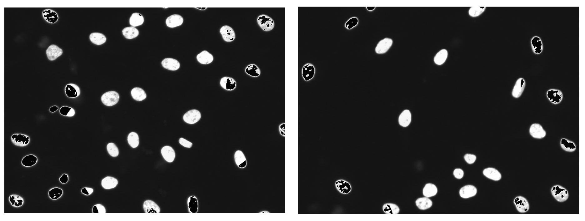
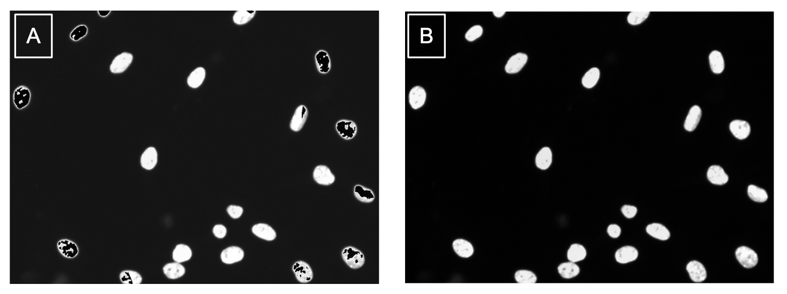
We have already implemented this multiple other projects!
Now, I am not going to sit here writing this blog and pretend like coSMicQC works without any fault.
I want to be very clear, this method is very good when applying it to cells without perturbation (e.g., happy, normal cells).
We applying coSMicQC to a dataset where there are cells treated with many different perturbations, we saw that nuclei with very interesting phenotypes ended up failing quality control (red) at a higher rate than those that looked more normal.</p>

<figure class="figure">
  <a class="figure_image" style="width: 100%;">
    <img src="/images/blog/cosmicqc/phenotype_example.png" alt="Example of passing (green) and failing (red) single cells for a normal phenotype FOV (left) and interesting phenotype FOV (right)." title="Example of passing (green) and failing (red) single cells for a normal phenotype FOV (left) and interesting phenotype FOV (right)." style="width: 100%;" loading="lazy" />
  </a><figcaption class="figure_caption">Example of passing (green) and failing (red) single cells for a normal phenotype FOV (left) and interesting phenotype FOV (right).
</figcaption></figure>

<p>This means that unfortunately, coSMicQC is not robust to some phenotypes and might over-correct the data.
But, quality control is not a perfect science.
The purpose of quality control, regardless of field, is to maximize the amount of poor quality cell removed while minimizing the amount of good quality cells being wrongly eliminated from the dataset.
This means that no matter what, you must expect some false positives, but we can attempt to control for this.</p>

<p>Given that we know the current limitations of the current simple methodology of coSMicQC, we are looking to improve by finding new methods to implement into our software.
Some of the current ideas we are thinking of testing include DBSCAN (proposed by Erik Serrano aka @axiomcura) and PCA or UMAP to utilize either all features or selected features to find outliers based on clusters.
As well, given the results from Rezvani et al., we might considering incorporating the HBOS method from the PyOD package into coSMicQC.</p>

<p>Our big goal for 2025 is publish a paper for coSMicQC, which means we will be testing on more datasets.
We plan on updating this blog with more sections that include the results from evaluating on more data, so please look out for more!</p>

<hr />

<h2 id="final-thoughts">Final thoughts</h2>

<p>If you have gotten to the end of this blog and have an idea that you want to propose, please feel free to <a href="https://github.com/WayScience/coSMicQC/issues">add an issue</a> to the coSMicQC GitHub!
We would really like to make a push towards standardizing this process within the traditional image-based profiling workflow.
We hope to build a community around single cell quality control for morphology profiles, so we can lead the field to a future with higher-quality datasets.</p>

<p>Thank you for reading, and happy profiling! 👩🏻‍💻</p>

<h3 id="acknowledgements">Acknowledgements</h3>

<p>Thank you to the Way Lab for their unwavering support!
A special thanks to Dave Bunten for his direct contributions to the software behind coSMicQC and dedication to improving data quality and standardization!
I would also like to thank Erik Serrano for his valuable contributions to the repository, specifically in documenting innovative ideas to advance the software and the process of single-cell quality control!</p>

<p>Figures were either generated in <a href="https://excalidraw.com/">Excalidraw</a> using emojis derived mainly from <a href="https://fonts.google.com/noto/specimen/Noto+Color+Emoji">Google’s emoji combiner tool</a>. 
One emoji was derived from <a href="https://emojis.sh/">AI Emoji Generator</a> (stage and curtains).</p>]]></content><author><name>Jenna Tomkinson</name></author><category term="opinions" /><category term="process" /><category term="software" /><category term="quality-control" /><summary type="html"><![CDATA[Let’s tour the single-cell morphological galaxy with coSMicQC!]]></summary></entry><entry><title type="html">Steps for Performing Illumination Correction in Microscopy Images</title><link href="/2023/08/07/illumsteps.html" rel="alternate" type="text/html" title="Steps for Performing Illumination Correction in Microscopy Images" /><published>2023-08-07T00:00:00+00:00</published><updated>2023-08-07T00:00:00+00:00</updated><id>/2023/08/07/illumsteps</id><content type="html" xml:base="/2023/08/07/illumsteps.html"><![CDATA[<h1 id="the-process-of-illumination-correction-on-microscopy-images">The Process of Illumination Correction on Microscopy Images</h1>

<p>Hello again! 👋</p>

<p>It has been a little while since <a href="https://www.waysciencelab.com/2022/11/01/segmentation.html">the last blog post</a>!
But, I am excited to be writing this new and updated blog post stemming from <a href="https://www.waysciencelab.com/2022/08/09/illumcorrect.html">my first blog post ever on illumination correction (IC)</a>.
I have grown and learned a lot in my first year of my position, from CellProfiler pipelines to multi-processing.
After all the experience I have gained, I believe it is the right time to make an updated blog post on the fun concept of illumination correction!</p>

<hr />

<h2 id="contents">Contents</h2>

<p>Within this blog post, I will be going over:</p>

<ol>
  <li>🪜 Basic steps to illumination correction</li>
  <li>💡 Overview on CellProfiler IC</li>
  <li>🎙️ An updated opinion on IC methods</li>
</ol>

<p><strong>Note:</strong> Data used as examples are as follows:</p>

<ol>
  <li><em>Sections 1 and 2:</em> <a href="https://cellprofiler.org/examples">Illumination correction example from CellProfiler</a></li>
  <li><em>Section 3:</em> <a href="https://github.com/WayScience/nf1_cellpainting_data/tree/main/0.download_data">Plate 1 data from the nf1_cellpainting_data repository</a></li>
</ol>

<hr />

<p>WAIT! ✋ Here is a quick recap:</p>

<p><strong>What is illumination correction?</strong></p>

<blockquote>
  <p>Illumination correction (IC) is the method of adjusting the lighting within a collection of images so that the lighting is evenly distributed across the image (no dim or bright spots).</p>
</blockquote>

<p>This is an important step within an image-based analysis pipeline since the uneven illumination in an image impacts segmentation performance and accuracy of intensity measurements.
Sometimes it is easy to see from the raw images that there is a need for illumination correction, but other times it might not be noticeable with the naked eye (Figure 1).</p>

<figure class="figure">
  <a class="figure_image" style="width: 100%;">
    <img src="/images/blog/illumsteps/fig_1.png" alt="" title="" style="width: 100%;" loading="lazy" />
  </a></figure>

<blockquote>
  <p><strong>Figure 1. Variation in identifying uneven illumination.</strong> In image A, it is clear to see that the bottom right of the image is brighter and dims as it reaches the top left of the image. In image B, it is very hard to tell with the naked eye if there is any uneven illumination.</p>
</blockquote>

<hr />

<h2 id="basic-steps-to-illumination-correction">Basic steps to illumination correction</h2>

<p>So, what do you do if you can not tell if your images need illumination correction or not?
Lets talk about step 1!</p>

<h3 id="step-1-brighten-the-image-with-fiji">Step 1: Brighten the image with Fiji</h3>

<p>The easiest way to tell if there is uneven illumination in images that are dim or it is just not obvious is to increase the brightness to the point where you can see.</p>

<p>The software that I find to be the best at this (among many other things) is <a href="https://imagej.net/software/fiji/.">Fiji</a>.</p>

<p>It is incredibly simple to use!
All you have to do is:</p>

<ol>
  <li>Open up Fiji</li>
  <li>Load in an image from your dataset</li>
  <li>Go to “Image -&gt; Adjust -&gt; Brightness/Contrast” (the shortcut on Mac and Linux is <code class="language-plaintext highlighter-rouge">Command + Shift + C</code>)</li>
  <li>Use the second bar to adjust the <code class="language-plaintext highlighter-rouge">maximum</code> brightness of the image and see what emerges</li>
</ol>

<p>Once the image is brightened, either you will see the illumination across the image to be even (e.g., as you increase to max brightness, the image will become entirely white) OR you will start to see one part of the image to be more bright than the rest (Figure 2).</p>

<figure class="figure">
  <a class="figure_image" style="width: 100%;">
    <img src="/images/blog/illumsteps/fig_2.png" alt="" title="" style="width: 100%;" loading="lazy" />
  </a></figure>

<blockquote>
  <p><strong>Figure 2. Increasing brightness improves ability to observe uneven illumination.</strong> Image A is the raw version of the image, where it is hard to tell if the image is suffering from uneven illumination. Image B is the brightened version of Image A, where it is much clearer to see that this image has a much brighter area in the lower right of the image.</p>
</blockquote>

<p>Now that we have identified that our image definitely needs to be corrected for uneven illumination, we will need to create an illumination correction function.
If you would like to go over how to make function in CellProfiler, please go to the <a href="https://www.waysciencelab.com/2023/08/07/illumsteps.html#creating-a-cellprofiler-ic-function">next section of the blog post</a>.
This section goes over the basics, so lets move on to step two!</p>

<h3 id="step-2-confirm-that-your-ic-function-worked">Step 2: Confirm that your IC function worked</h3>

<p>Once you have performed the illumination correction method of your choosing, now you should probably confirm that it even worked!</p>

<p>Currently, there is no automatic or exact quantitative way to determine if the IC method worked on your dataset.
You can probably use ChatGPT and it will tell you to measure the contrast of the image or standard deviation of the pixel intensities in the image, but I find this to be more tedious and does not always work.</p>

<p>The most full-proof method I have found is exactly what I have already told you!
Brighten up the image and see how the illumination looks across the image.
What you expect to see is that your IC corrected images will have even illumination across the image and no brighter areas (Figure 3).</p>

<figure class="figure">
  <a class="figure_image" style="width: 100%;">
    <img src="/images/blog/illumsteps/fig_3.png" alt="" title="" style="width: 100%;" loading="lazy" />
  </a></figure>

<blockquote>
  <p><strong>Figure 3. Illumination correction improves contrast and evens illumination.</strong> In panel A, it demonstrates how uneven the illumination is when brightened with the decreased contrast between the foreground (organelles) and the background. In panel B, the image raw image has been corrected and it is noticeable that the organelles are less intense. When brightened, it is more noticeable that the contrast is improved and the illumination across the image is even.</p>
</blockquote>

<h3 id="step-3-repeat-for-each-channel">Step 3: Repeat for each <em>channel</em></h3>

<p>For all datasets you work with, these basic steps should be taken as quality control assurance prior to analysis.</p>

<p>Traditionally, an IC function is created for each <code class="language-plaintext highlighter-rouge">channel</code>, not all of the images in a dataset.
This is due to different distributions and sizes of the objects in a channel.
I have also noticed that patterns of uneven illumination tend to be channel specific.</p>

<p>If these steps are not performed and images are left with uneven illumination, you will likely have a hard time finding optimal segmentation parameters and the intensity measurements will not be biologically accurate.</p>

<p><strong>NOW</strong> that you know the steps to determining if IC is needed and/or if an IC method worked, lets get into how to create an IC function through CellProfiler!</p>

<hr />

<h2 id="creating-a-cellprofiler-ic-function">Creating a CellProfiler IC function</h2>

<p>You might be thinking: “Well, you already said that you are using images from an already existing tutorial from CellProfiler, why do you need to create <em>ANOTHER</em> tutorial?”.</p>

<p>Well, good question! I have two main reasons:</p>

<ol>
  <li>That tutorial is from 2011, when CellProfiler was in version 2.0. As of this blog post, the latest version of CellProfiler is v4.2.5, and <strong>MANY</strong> things have changed since then.</li>
  <li>The tutorial is more specific to the datasets they are using, and for me, I find it to be too narrow and doesn’t go into as much detail on the specific parameters as I would like.</li>
</ol>

<p><strong>Please note that I do not think that this tutorial is bad in anyway.</strong>
My hope with this blog post is to make a more concise and broader version of this tutorial.</p>

<p>Now that the logistics are out of the way, lets get into making an IC function in CellProfiler!</p>

<h3 id="correctilluminationcalculate-module">CorrectIlluminationCalculate Module</h3>

<p>The module to create the IC function is known as <code class="language-plaintext highlighter-rouge">CorrectIlluminationCalculate</code>.
This will create the function but will not apply it to the images.
To apply it to the images, you will use the second module in this duo, <code class="language-plaintext highlighter-rouge">CorrectIlluminationApply</code>, but we will get to that later.</p>

<p><strong>BIG NOTE:</strong> You will need to have one module per channel (e.g., 3 channel = 3 modules).</p>

<p>There are <strong>A LOT</strong> of parameters in this module where for first time users like I myself was back a year ago, it can be pretty overwhelming.
In this blog, I am going over the most basic steps and parameters that I have found I use or change from the default most often.</p>

<h4 id="step-1-select-a-method-for-calculating-the-ic-function">Step 1: Select a method for calculating the IC function</h4>

<p>The first thing that you will need to decide when making a function is which method of calculating the function to use:</p>

<ol>
  <li><strong>Regular:</strong> Recommended per CellProfiler to use on a dataset where for majority of the objects in an image are evenly dispersed and covers most of the image (e.g., little background area). This method will create the function based on each pixel in an image.</li>
  <li><strong>Background:</strong> Recommended per CellProfiler to use on a dataset where based on the images, the pattern of uneven illumination is the same between the background and objects. I personally have found that this can be hard to tell and it takes trial and error to find if this method works best on your dataset. This method finds the minimum pixel intensity in multiple “blocks” that set across the image.</li>
</ol>

<p>When using the <strong>Regular</strong> method, make sure that <code class="language-plaintext highlighter-rouge">Rescale the illumination function</code> is turned on since this is a required parameter.
This is the <em>opposite</em> for the <strong>Background</strong> method.
Make sure that this same parameter is <strong>turned off</strong>, or it will cause this function to break and produce bad results.</p>

<p>The last parameter to note when using the <strong>Background</strong> method is the <code class="language-plaintext highlighter-rouge">Block size</code> parameter.
This parameter is specific to this method and you will set a pixel value.
This block, as referenced above, is placed multiple times to cover the image.
The value you should use is one where the block is most likely to have background and not objects.
I have found this takes trial and error to find the optimal value, but I recommend trying the default first.</p>

<h4 id="step-2-determine-how-the-selected-ic-function-is-calculated">Step 2: Determine how the selected IC function is calculated</h4>

<p>There are three options here to choose from:</p>

<ol>
  <li><strong>Each:</strong> Calculate an IC function per image in a group of images (e.g., channel)</li>
  <li><strong>All: Across Cycles:</strong> Calculate an IC function based on all images in a group which will finish during the last cycle, which means you can flag and remove images in the <code class="language-plaintext highlighter-rouge">FlagImage</code> module.</li>
  <li><strong>All: First Cycle:</strong> Calculate the IC function based on all images in a group during the first cycle, which means that you will not be able to filter out any images.</li>
</ol>

<p><strong>Note:</strong> I will be completely honest here, I don’t really know what the big difference is between the <em>All</em> methods other than the ability to filter images.
Calculating the function after the first or last cycle doesn’t seem like a big difference to me, but I could be wrong.</p>

<p>Depending on the pipeline, I normally use either <strong>Each</strong> or <strong>All: Across Cycles</strong>.
I normally use the <strong>Each</strong> method when I want to save all of my corrected images at the end of the pipeline, while I use <strong>All: Across Cycles</strong> when I want to save the IC function as an <code class="language-plaintext highlighter-rouge">.npy</code> file to use in the next downstream pipeline (e.g., segmentation and feature extraction).</p>

<h4 id="step-3-pick-the-smoothing-method">Step 3: Pick the smoothing method</h4>

<p>I won’t put down all of the different smoothing methods you can use here in this blog, or we would be here all day!
<a href="https://github.com/CellProfiler/CellProfiler/blob/8e2c86445a5bb406cd9d5fd124f87a036b7ec51b/cellprofiler/modules/correctilluminationcalculate.py#L287">Here</a> is the link to the source code from CellProfiler that goes through the documentation for each method.</p>

<p>The method I typically choose for all of my IC pipelines is (drum roll please! 🥁):
<strong>FIT POLYNOMIAL</strong></p>

<p>Though it doesn’t sound very exciting, I assure you it is!
This method I have found to be the most robust and produce pretty decent results.
Though it isn’t perfect sometimes, I find this method to consistently improve the illumination in my various image sets compared to the other methods.</p>

<p><strong>BUT…</strong>
Take my advice with a grain of salt.
I am only discussing what has been the method that consistently works the best for me with my data that contains different cell lines taken from different microscopes.
This can definitely be different for your dataset, so I recommend playing around with this parameter as you are testing.</p>

<h4 id="testing-testing-testing">TESTING, TESTING, TESTING</h4>

<p>Rinse and repeat the above steps with different parameters to see what sticks!
I didn’t go over <em>EVERY</em> parameter that is offered in this module, so it is on you to determine what parameters are relevant to getting the best possible function.</p>

<h3 id="correctilluminationapply-versus-saveimages-module">CorrectIlluminationApply versus SaveImages module</h3>

<p>Now that an illumination correction function has been created, you have two options:</p>

<ol>
  <li>If you decided to use the <strong>Each</strong> method, then it would be best to apply the correction onto your images and save them in the same pipeline with the <code class="language-plaintext highlighter-rouge">CorrectIlluminationApply</code> module. <strong>IMPORTANT:</strong> You will need to make sure the method for the <code class="language-plaintext highlighter-rouge">Select how the illumination function is applied</code> parameter matches the method from the previous module. To be exact, if you use applied the <strong>Regular</strong> method, you use <strong>Divide</strong> to apply the function. If you use <strong>Background</strong>, you use <strong>Subtract</strong>.</li>
  <li>If you used an <strong>All</strong> method, the documentation from CellProfiler mentions that you can save the illumination function with the <code class="language-plaintext highlighter-rouge">SaveImages</code> module. I would highly recommend this when you are planning on correcting the images during the next pipeline and don’t want to have the intermediate files (e.g., corrected images). When saving the IC functions, make sure you are saving them as <code class="language-plaintext highlighter-rouge">Images</code> in the <code class="language-plaintext highlighter-rouge">npy</code> file format (you can thank me later!).</li>
</ol>

<hr />

<p>And VIOLA! ✨</p>

<p>You now created your illumination correction pipeline in CellProfiler and you know exactly how to make sure that you made the best possible function for your dataset!</p>

<p>Feel free to checkout my GitHub profile and look into the image-based analysis repositories I am working on for examples of illumination correction pipelines I have made: <a href="https://github.com/jenna-tomkinson">jenna-tomkinson GitHub profile</a></p>

<hr />

<h2 id="updated-opinions-on-ic-software">Updated opinions on IC software</h2>

<p>Now, I believe it is the right time to go back and reflect on my opinions regarding three different illumination correction methods I discussed in <a href="https://www.waysciencelab.com/2022/08/09/illumcorrect.html">my first IC blog</a>.</p>

<p>To refresh your memory, I went over these three software; CellProfiler, PyBaSiC, and CIDRE.</p>

<p><strong>Note:</strong> I will not be including a section in the blog for CIDRE since it is still deprecated and can not be used.
This means I have nothing new to add, but I will still say that maintaining and even creating software takes a lot of work, so kudos to all of the software and their respective developers I mention in this blog.</p>

<p>In this portion of the blog, I will be going over:</p>

<ol>
  <li>CellProfiler</li>
  <li>BaSiCPy (formerly PyBaSiC)</li>
  <li>Comparison between methods</li>
</ol>

<p>Now that we have established our topics, lets go into each of them one by one!
As mentioned above, I will use the <a href="https://github.com/WayScience/nf1_cellpainting_data">nf1_cellpainting_data</a> repository for a comparison of the methods on the same dataset from .</p>

<h3 id="cellprofiler">CellProfiler</h3>

<p>This section will be short, sweet, and to the point:</p>

<p><strong>CellProfiler illumination correction has become my #1 go-to method! 🥇</strong></p>

<p>My one main complaint from my first blog was that there were way too many parameters.
This is a gripe I have with any software, as in my opinion, it becomes a big barrier for entry and makes it intimidating for unexperienced individuals to work with.
Over time and lots of trial and error, I became much more confident, learning many different tips and tricks along the way.
That is why my opinion has changed so much because I found <strong>when you know the most important parameters</strong>, it is the easiest method out of all three to test and determine the best function.</p>

<p>Along with making the function, being able to process images and correct them is the most streamlined and simple in CellProfiler.
Depending on the pipeline, all you need is a few modules and press the <code class="language-plaintext highlighter-rouge">Analyze</code> button.
As well, you have a ton of control over the output of the function or corrected images, and can insure the correct bit-depth, file format, etc.</p>

<p>CellProfiler is the standard in the image-based analysis field and will be hard to beat! 🥊
That is why I have dedicated an entire section to how you would make an IC function using CellProfiler and not any other method.</p>

<h3 id="basicpy-previously-pybasic">BaSiCPy (previously PyBaSiC)</h3>

<p>This package has gone through many big changes, including the name!
The difference was a bit jarring, as I ran into troubles when trying to implement the same code I had using for the previous version.</p>

<p>When attempting to test with this method in January, I struggled to get the process to work on even one image (see <a href="https://github.com/peng-lab/BaSiCPy/issues/120">issue #120</a> which is closed).
Now, 7 months later as I am writing this blog, I decided to go back and see if I could figure out what I did wrong.
Well, firstly, I now realized that all I needed was to turn my directory of images into a list of numpy arrays (silly me! 😜).
There seems to be no current way to only run on one image (also noted in <a href="https://github.com/peng-lab/BaSiCPy/issues/104">issue #104</a>), which is fine, but good to keep in mind.
Now with my new and improved skills compared to me 7 months ago, I decided to take another crack at BaSiCPy in Python.</p>

<p><strong>Note:</strong> To be specific, this was the code that I used to create IC function with BaSiCPy (based off of the <a href="https://github.com/peng-lab/BaSiCPy/blob/dev/docs/notebooks/WSI_brain.ipynb">WSI_brain example notebook</a>):</p>

<div class="language-python highlighter-rouge"><div class="highlight"><pre class="highlight"><code><span class="c1"># set the function, removed smoothness_flatfield=1 which is default
</span><span class="n">basic</span> <span class="o">=</span> <span class="nc">BaSiC</span><span class="p">(</span><span class="n">get_darkfield</span><span class="o">=</span><span class="bp">True</span><span class="p">)</span>
<span class="n">basic</span><span class="p">.</span><span class="nf">fit</span><span class="p">(</span><span class="n">images</span><span class="p">)</span>

<span class="c1"># correct the images
</span><span class="n">images_transformed</span> <span class="o">=</span> <span class="n">basic</span><span class="p">.</span><span class="nf">transform</span><span class="p">(</span><span class="n">images</span><span class="p">)</span>
</code></pre></div></div>

<p>Good news!
I was able to get it to work! 🎉
<strong>But…</strong></p>

<p>I want to make clear something <strong>very important</strong>.
Make sure that you are using the recommended function from BaSiCPy to save the images, which is <code class="language-plaintext highlighter-rouge">skimage.io.imsave</code>.</p>

<p>At first, I attempted to use the <code class="language-plaintext highlighter-rouge">pillow</code> package to convert the images from numpy arrays and save the images with the <code class="language-plaintext highlighter-rouge">Image.save</code> function.
I will admit, this was something that ChatGPT recommended for saving images from numpy arrays.
What occurred was VERY interesting.
Some images showed black/empty spots which I call “artifacts” (Figure 4).</p>

<figure class="figure">
  <a class="figure_image" style="width: 100%;">
    <img src="/images/blog/illumsteps/fig_4.png" alt="" title="" style="width: 100%;" loading="lazy" />
  </a></figure>

<blockquote>
  <p><strong>Figure 4. Artifacts produced when using the pillow package to save images.</strong> Compared to other images with different organelles, these artifacts are disproportionately produced in the nuclei channel. As well, the artifacts become more intense in images where organelles were highly saturated.</p>
</blockquote>

<p>After this issue, I decided to take a look back at how I had saved the images when using the older version of BaSiCPy (see notebook from old repository <a href="https://github.com/WayScience/Benchmarking_NF1_data/blob/main/1_preprocessing_data/PyBaSiC_Pipelines/Illumination_Correction_Plate1.ipynb">here</a>).
I had in fact used the <code class="language-plaintext highlighter-rouge">skimage</code> package to save the images, but I had converted the images to 8-bit which was different from the original images bit-depth for that dataset (which was 16-bit).
I found out this was due my oversight when implementing the code from another repository that this conversion occurring was a different bit-depth than my original images (see <a href="https://github.com/WayScience/Benchmarking_NF1_data/issues/44">the issue</a> I created and recently updated).
Though embarrassing, I am realizing that I had to make this mistake to be able to learn and greater appreciate the small details of code and working with images.
Now going back and having more knowledge under my belt, I was able to identify this problem and implement the correct conversion to 16-bit.
Comparing the same images when using the different saving methods, I can say that using <code class="language-plaintext highlighter-rouge">skimage.io.save</code> was a success (Figure 5)!</p>

<figure class="figure">
  <a class="figure_image" style="width: 100%;">
    <img src="/images/blog/illumsteps/fig_5.png" alt="" title="" style="width: 100%;" loading="lazy" />
  </a></figure>

<blockquote>
  <p><strong>Figure 5. Method of output impacts quality of images.</strong> (a) This corrected image was saved using the PIL Image function which caused issues in the image like the black artifacts in the nuclei. (b) This corrected image was saved using the recommended scikit-image package and the results are free from artifacts.</p>
</blockquote>

<p>You might wonder: “Well, why even need to convert in the first place?”</p>

<p>Great question!
If you don’t convert and just save the corrected image straight from BaSiCPy, your image will be a 32-bit image.
Now, I am not an expert in bit-depth at all.
From what I understand, having higher bit-depth means more information preserved in the image.
But, I am not sure how more information would be added into a image that was a lower bit-depth to begin with.
So, in my opinion, it makes sense to convert the corrected images back to the original bit-depth to preserve the same amount of information that was originally collected.</p>

<p>Since one of my biggest issues was that an output method wasn’t added into <a href="https://github.com/peng-lab/BaSiCPy/tree/dev/docs/notebooks">the BaSiCPy repository example notebooks</a>that are linked in the main README, I decided to contribute with <a href="https://github.com/peng-lab/BaSiCPy/pull/132">my first PR for the repo</a>!
I implemented the code I had to output corrected images into all the notebook and included extra notes to make the process of using BaSiCPy more interpretable.
My hope is that this will make it much easier for someone new to this package to be able to quickly use it without going through all the troubles I did.</p>

<p>So, moment of truth…
Will I end up including this in my pipelines over CellProfiler?</p>

<p>My answer is unfortunately no at this time.</p>

<p>I have identified a few limitations that influenced why I am not going to use it over CellProfiler for my traditional image-based analysis projects:</p>

<ol>
  <li>It is not optimal for running with multiple channels. A way around this could be to utilize a Python package called <a href="https://papermill.readthedocs.io/en/latest/">papermill</a>, which allows for running one notebook with different variables through an <code class="language-plaintext highlighter-rouge">sh</code> file (<a href="https://github.com/WayScience/pyroptosis_signature_data_analysis/blob/main/1.Exploratory_Data_Analysis/correlation_run.sh">here</a> is an example showing how this is done with two different variables).</li>
  <li>There isn’t a way to run multiple plates a time (e.g., parallel) with this method, unlike compared to CellProfiler (<em>wink, wink; will talk about in the next blog</em> 😉). Being able to run multiple plates at once decreases the computational time, which can be important for some projects.</li>
</ol>

<p><strong>BUT!</strong>
I haven’t had a project that included time lapse data, so I will definitely be taking on the challenges I mentioned above with the time comes.</p>

<h4 id="side-note">Side note</h4>

<p>This method of illumination correction is not just a Python package. This has been implemented as plugins for:</p>

<ol>
  <li><strong><a href="https://imagej.net/software/fiji/">ImageJ/Fiji</a></strong>: https://github.com/marrlab/BaSiC</li>
  <li><strong><a href="https://napari.org/stable/">Napari</a></strong>: https://github.com/peng-lab/napari-basicpy</li>
</ol>

<p>I have not been able to test either of these plugins.</p>

<p>Firstly, I have not tested the ImageJ plugin due to seeing that as of last month in <a href="https://github.com/marrlab/BaSiC/issues/4">an issue</a>, one of the developers stated this plugin is no longer maintained.
The issue references that there is no command for <code class="language-plaintext highlighter-rouge">BaSiC</code>, which is one of the big functionality changes made in the recent update.
Since this plugin has been around for a while, it likely means that it has not been updated to use the new version of BaSiCPy.</p>

<p>Lastly, I have not tested with the napari plugin as was planning on testing with this new software on my MacBook, which uses a M2 Pro chip.
If you don’t know, the M1 and M2 chips come with <strong>MANY</strong> issues when trying to use some software packages due to lack of support.
Unfortunately, this is more of an Apple issue it seems than a developer issue, so I just don’t currently have the bandwidth to try and test out the software and plugin on my Linux machine (the powerhouse of a computer the lab calls <code class="language-plaintext highlighter-rouge">fig</code> 🍃).</p>

<h3 id="comparison-of-methods">Comparison of methods</h3>

<p>Though I have already stated that I will be used CellProfiler over BaSiCPy for usability reasons, I wanted to include a direct comparison of the quality of correction from both methods (Figure 6).</p>

<figure class="figure">
  <a class="figure_image" style="width: 100%;">
    <img src="/images/blog/illumsteps/fig_6.png" alt="" title="" style="width: 100%;" loading="lazy" />
  </a></figure>

<blockquote>
  <p><strong>Figure 6. Comparing quality of illumination correction between methods.</strong> All images are brightened to approximately the same level as seen in the value in the red circle (+/- 50 units). The corrected image from BaSiCPy looks to have made the illumination more even by correcting the bright spot in the middle of the raw image, but did not improve the contrast between the foreground and background. CellProfiler is able to both even out the illumination across the image and significantly improve the contrast.</p>
</blockquote>

<p>I can say that without a doubt that CellProfiler (with optimal parameters found through trial and error) is able to significantly outperform PyBaSiC.
The most significant difference is with the contrast, which is important to improve segmentation as low contrast can cause issues with any segmentation software to identify organelles in the foreground versus the background.</p>

<hr />

<h2 id="conclusion">Conclusion</h2>

<p>The main takeaway that I hope that all readers can take from this blog is that illumination correction is a skill and it takes time to get used to the process.
As well, it is important to know all the tools 🛠️ at your disposal to choose what is the best method for your dataset.</p>

<p>I really hope that this blog will help make the process of illumination correction easier, even if it is just for one person.
I know I would have benefited from something like this when I first started.
I think the past version of myself would approve of this, if I do say so myself! 🤗</p>]]></content><author><name>Jenna Tomkinson</name></author><category term="opinions" /><category term="process" /><summary type="html"><![CDATA[The Process of Illumination Correction on Microscopy Images]]></summary></entry><entry><title type="html">Segmentation Software Usability and Performance: Part I</title><link href="/2022/11/01/segmentation.html" rel="alternate" type="text/html" title="Segmentation Software Usability and Performance: Part I" /><published>2022-11-01T00:00:00+00:00</published><updated>2022-11-01T00:00:00+00:00</updated><id>/2022/11/01/segmentation</id><content type="html" xml:base="/2022/11/01/segmentation.html"><![CDATA[<h1 id="a-brief-comparison-of-popular-cell-segmentation-software">A Brief Comparison of Popular Cell Segmentation Software</h1>

<p>Welcome back! I hope that you were able to come up with an amazing illumination correction pipeline from <a href="https://www.waysciencelab.com/2022/08/09/illumcorrect.html">my illumination correction blog post</a> and are ready for segmentation! 
If you are just starting with this blog post, then welcome in!</p>

<p>As a reminder from my previous post, keep in mind that any method or software you use in your pipeline might not be optimal or might not contain the functionalities that you want (e.g. model training, etc.). 
I recommend benchmarking different methods with your own data.</p>

<p>I will be comparing multiple segmentation methods in this blog post, which are:</p>

<ol>
  <li>
    <p>CellProfiler</p>
  </li>
  <li>
    <p>Cellpose</p>
  </li>
  <li>
    <p>Cellpose plugin for CellProfiler</p>
  </li>
</ol>

<p>I also tested Ilastik, Weka Trainable Segmentation, and Scikit testing.
From my experience, these performed sub-optimally with my data. I will discuss these methods in part II of my segmentation blog.</p>

<p><strong>Note:</strong> My segmentation findings in this blog are based on Cell Painting data. 
For more information on Cell Painting assays and what makes them unique, see the following <a href="https://github.com/carpenterlab/2022_Cimini_NatureProtocols/wiki#morphological-image-feature-extraction-from-microscopy-data">GitHub wiki</a> from the Broad Institute.</p>

<h2 id="cellprofiler">CellProfiler</h2>

<p>CellProfiler might have been difficult to work with for illumination correction, but CellProfiler excels in segmentation. The standard segmentation pipeline for Cell Painting images with CellProfiler is as follows:</p>

<ol>
  <li>
    <p><code class="language-plaintext highlighter-rouge">IdentifyPrimaryObjects</code>: Segment nuclei from a DAPI/Hoechst channel</p>
  </li>
  <li>
    <p><code class="language-plaintext highlighter-rouge">IdentifySecondaryObjects</code>: Segment whole cells using an RNA channel</p>
  </li>
  <li>
    <p><code class="language-plaintext highlighter-rouge">IdentifyTertiaryObjects</code>: Segment cytoplasm by subtracting the nuclei from the whole cell outline</p>
  </li>
</ol>

<h3 id="identifying-primary-objects-nuclei">Identifying primary objects (nuclei)</h3>

<p>Starting with the IdentifyPrimaryObjects module, our goal is to identify the nuclei in the DAPI or Hoechst images. 
When first applying the pipeline, this module does not show the “advanced settings”, which makes it more approachable. 
The only parameters you need to set are the minimum and maximum diameters of the objects, which is easy to do.
Following the steps in this <a href="https://youtu.be/eriZdORpFxs?t=715">tutorial video</a>, a user can easily approximate the pixel size of the nuclei in an image.</p>

<p>But, just changing this individual parameter does not work for every dataset. 
So, it is more optimal to select <code class="language-plaintext highlighter-rouge">yes</code> and change parameters within the advanced settings (yay… more prototyping…). 
<strong>BUT!</strong>
And I mean but! 
I found that the manual parameters in this segmentation module were very easy to work with. 
You can see the impact of each parameter through the <code class="language-plaintext highlighter-rouge">Test Mode</code> feature.</p>

<p>I will be honest; IdentifyPrimaryObjects is the second easiest part of the whole segmentation pipeline. 
Nuclei are very easy to segment and there are not many necessary parameter changes other than setting the maximum and minimum diameter of the nuclei.</p>

<h3 id="identifying-secondary-objects-cells">Identifying secondary objects (cells)</h3>

<p>In contrast, IdentifySecondaryObjects was the hardest of the three steps. 
This was because in our data (we’re working with Schwann cells), the actin from the RFP channel (used for segmenting the whole cell), is very long and stringy. 
The atypical shape of Schwann cell actin makes it harder for CellProfiler to segment each cell (see figures below).</p>

<p>In this module, I changed many parameters to optimize segmentation. 
For my data, the most important parameters are:</p>

<ol>
  <li>
    <p>Method to identify secondary objects</p>
  </li>
  <li>
    <p>Thresholding method</p>
  </li>
  <li>
    <p>Threshold correction factor</p>
  </li>
</ol>

<p>For example, the method that you choose for identifying secondary objects can make a dramatic difference in segmentation (Figure 1).</p>

<figure class="figure">
  <a class="figure_image" style="width: 100%;">
    <img src="/images/blog/segmentation/identification_method_blog.png" alt="" title="" style="width: 100%;" loading="lazy" />
  </a></figure>

<blockquote>
  <p>Figure 1. Comparison of methods for identification of secondary objects. This figure demonstrates how important the chosen method for identification is for cell segmentation. As you can see in the <code class="language-plaintext highlighter-rouge">Watershed -- Image method</code> (right), it incorrectly segments the maroon-colored cell in the top right box by giving it a long arm (red arrow) that should be a part of a different cell. But, in the <code class="language-plaintext highlighter-rouge">Propagation method</code> (left), it segments the light orange-colored cell correctly and does not segment the cell next to it where it contains parts of the orange-colored cell.</p>
</blockquote>

<p>But no matter what parameter you choose, there is always a “give and
take”. For example, when choosing a value for the threshold correction
factor (TCF), one value can segment one cell better than the other while
the other value segments a different cell better (Figure 2).</p>

<figure class="figure">
  <a class="figure_image" style="width: 100%;">
    <img src="/images/blog/segmentation/tcf_fig_blog.png" alt="" title="" style="width: 100%;" loading="lazy" />
  </a></figure>

<blockquote>
  <p>Figure 2. Comparison of threshold correction factor values (TCF). This figure shows how complicated picking a TCF value is to optimize segmentation. In the left panel, I set the TCF to 1.5, which segments the dark blue cell (green arrow) correctly but under segments the light green cell (red arrow). In the right panel, the TCF is 0.6, which segments the light blue cell (light green cell from the left panel) correctly, not leaving out any parts. In contrast, TCF=0.6 under segments the dark blue cell (same as the other panel), artificially adding some of its actin to the cell to its right. I used the same segmentation method for both panels.</p>
</blockquote>

<p>As you can see, the main reason why this module is so hard is that it is very difficult to find the best parameters. 
But like with the IdentifyPrimaryObjects, this module is very easy to prototype and make changes to the parameters to get the best possible results.</p>

<h3 id="identifying-tertiary-objects-cytoplasm">Identifying tertiary objects (cytoplasm)</h3>

<p>Lastly, the IdentifyTertiaryObjects module is the easiest to work with out of all the steps. 
All you have to do is select the <code class="language-plaintext highlighter-rouge">Cells</code> object for the larger identified objects and the <code class="language-plaintext highlighter-rouge">OrigNuclei</code> (or however you called the objects from the IdentifyPrimaryObjects module) for the smaller identified objects. 
Then, give the new tertiary object the name <code class="language-plaintext highlighter-rouge">Cytoplasm</code>, and you are done!</p>

<p>I believe that CellProfiler is a great segmentation option for my project. 
It did an amazing job segmenting the small stringy parts of the cells, which is likely to fully capture the cells’ morphology.</p>

<p>I will be using a CellProfiler pipeline for segmentation and feature extraction (hint, hint for the next blog post 😉). 
CellProfiler has many different parameters and methods to use, which makes it robust for multiple types of data sets. 
Segmentation is one feature of CellProfiler where it shines brightest.</p>

<h2 id="cellpose-20">Cellpose 2.0</h2>

<p>Now it is time to talk about the software that cell image biologists have raved over all across Twitter.</p>

<p>Cellpose is a software that focuses on segmentation and is described as a “generalist algorithm”. 
It has a GUI that is very helpful for prototyping and can be implemented in Python.</p>

<p>Unlike CellProfiler, Cellpose does not have the ability to segment out multiple objects in one run. 
Instead, it provides different pre-trained models to perform segmentation for one specific object per run. 
For Cell Painting data, our lab decided on segmenting nuclei followed by whole cells (which we also call cytoplasm interchangeably).</p>

<p>The best part of Cellpose is, in my opinion, that only three out of all the parameters made a difference in my data (depending on the object that you are trying to segment). 
These are:</p>

<ol>
  <li>
    <p>Cell Diameter (in pixels)</p>
  </li>
  <li>
    <p>Flow threshold</p>
  </li>
  <li>
    <p>Model</p>
  </li>
</ol>

<p>Cell diameter is so important because if set too large, it could over-segment objects (e.g. include background or merge cells). 
But set too small, it will incorrectly segment a bunch of small regions within the object instead of segmenting it whole. (Figure 3)</p>

<figure class="figure">
  <a class="figure_image" style="width: 100%;">
    <img src="/images/blog/segmentation/cell_diameter_blog.png" alt="" title="" style="width: 100%;" loading="lazy" />
  </a></figure>

<blockquote>
  <p>Figure 3. Comparison of cell diameter (CD) impact on segmentation. This figure demonstrates how CD values can make a big impact on how Cellpose segments nuclei. The left panel shows what happens when the CD is very low (segmenting nuclei into multiple parts) and the right panel shows what happens when the CD is very high (combining nuclei with other cells or artifacts). CD was the most important parameter that I toggled when optimizing nuclei segmentation.</p>
</blockquote>

<p>There are multiple <a href="https://cellpose.readthedocs.io/en/latest/models.html">models</a> that you can use for segmentation. 
You can use any model, but the three models that I found most useful for my data were: <code class="language-plaintext highlighter-rouge">nuclei</code>, <code class="language-plaintext highlighter-rouge">cyto</code>, and <code class="language-plaintext highlighter-rouge">cyto2</code>. 
During prototyping, I used each of these to see which segmented nuclei and whole cells better. 
In the end, I found <code class="language-plaintext highlighter-rouge">cyto</code> worked best with nuclei and <code class="language-plaintext highlighter-rouge">cyto2</code> worked best with whole cells.</p>

<p>As I was attempting to segment whole cells from my project, I noticed that Cellpose struggled when you only provided the actin channel. 
It could not determine where cells were since it did not have a nucleus channel to reference.</p>

<p>In Cellpose 2.0, there isn’t a way for you to load a group of images from multiple channels and use the nucleus channel as the base for segmenting other channels. 
You would need to create composite images (RGB) from each site to be able to reference the nucleus channel. 
That takes an extra step, which is what I have done in <a href="https://github.com/jenna-tomkinson/NF1_SchwannCell_data/blob/548983b6cd32ed4121e719e34eb84934185ae0c6/2_segmenting_data/segmentation_utils.py#L67">my code for segmentation</a>.
This function overlays the channels for every site to then use as an input for running Cellpose headless through Python.</p>

<p>As seen in Figure 4, Cellpose needs to have reference nuclei to accurately segment the cells in an image.</p>

<figure class="figure">
  <a class="figure_image" style="width: 100%;">
    <img src="/images/blog/segmentation/one_vs_composite.png" alt="" title="" style="width: 100%;" loading="lazy" />
  </a></figure>

<blockquote>
  <p>Figure 4. Segmentation comparison between one channel versus a composite image. This figure demonstrates the struggle Cellpose has with segmenting whole cells without reference nuclei. The middle image shows poor segmentation when lacking reference nuclei. When Cellpose has a composite image with all the channels, it is able to segment all of the whole cells and do it accurately (right).</p>
</blockquote>

<p>As well, I like how Cellpose can use GPU to run over CPU, which is way faster and more convenient when prototyping. 
This enables me to simultaneously use my CPU power for other tasks while I have Cellpose running through my GPU. 
You will need to properly <a href="https://github.com/MouseLand/cellpose\#gpu-version-cuda-on-windows-or-linux">install PyTorch</a> for this to work or it will run off of your CPU.</p>

<p>I really liked using Cellpose 2.0, mainly because there were fewer parameters for me to worry about, and it was very fast to prototype. 
I do wish that you could get outputs right from the GUI, but that is not necessary. 
For multiple projects within the lab, we use Cellpose 2.0 through Python to return center x and y coordinates for each cell in an image to use in analysis downstream. 
Unlike with CellProfiler, we do not use the GUI for running image analysis pipelines, but do use it for prototyping.</p>

<p>In all, I think that Cellpose is a great method for segmentation and has a lot of potential for use with diverse datasets with the ability to create your own models.</p>

<h2 id="cellpose-plugin-for-cellprofiler">Cellpose Plugin for CellProfiler</h2>

<p>Now, it’s the moment we have all been waiting for. 
Let’s talk about the Cellpose plugin for CellProfiler!</p>

<p>I had a lot of struggles with trying to get this to work on both my Linux computer and Macbook. 
I struggled to download CellProfiler from source, following many of the tutorials from the <a href="https://github.com/CellProfiler/CellProfiler/wiki">CellProfiler wiki on Github</a>.</p>

<p>After all of my struggles, I was able to install CellProfiler from source and install this plugin on my Linux computer (unfortunately, my Macbook to this day still refuses to just download CellProfiler from source). 
After installation, it only took one additional simple answer.
With the help of the amazing Beth Cimini, (she <a href="https://github.com/CellProfiler/CellProfiler/blob/master/cellprofiler/data/help/other_plugins.rst">linked me to a part of the wiki</a> that discussed setting CellProfiler plugin paths), I was able to use the plugin.</p>

<p>However, using the plugin came with an interesting challenge.</p>

<p>The challenge that I ran across was that my version of the <code class="language-plaintext highlighter-rouge">runcellpose.py</code> file was not displaying all the parameters that I saw on the version in the <a href="https://github.com/CellProfiler/CellProfiler-plugins/blob/master/runcellpose.py">CellProfiler-plugins repository</a>.
For the longest time, I believed that the file I downloaded onto my computer was the most up-to-date. 
When I finally thought, “<em>huh, maybe I should check my file and see what it looks like</em>”, I came to the realization that the code in my file did not match what was on the latest Github version.</p>

<p>Now, how could that be?! 
I have had that file downloaded since I first viewed the article about the plugin. 
Well, if you go <a href="https://forum.image.sc/t/new-cellprofiler-4-plugin-runcellpose/56858">the article</a> announcing the plugin, the link to the <code class="language-plaintext highlighter-rouge">runcellpose.py</code> file they provide is to the original one from 2021. 
I had assumed that this link was to whatever file was up to date, but that was incorrect.</p>

<p>Once I downloaded the most recent version of the plugin and put it in the plugins folder, the module for the plugin in CellProfiler had every parameter and model that I would have in Cellpose 2.0 (Figure 5).</p>

<figure class="figure">
  <a class="figure_image" style="width: 100%;">
    <img src="/images/blog/segmentation/cellpose_plugin_cp.png" alt="" title="" style="width: 100%;" loading="lazy" />
  </a></figure>

<blockquote>
  <p>Figure 5. Cellpose 2.0 parameters available in the CellProfiler Cellpose plugin. This figure demonstrates that the most up-to-date plugin file does work in CellProfiler and provides parameters (YAY!).</p>
</blockquote>

<p>Since I had so many issues with the install, and when you look up “Cellpose plugin for CellProfiler” on Google, it pulls up the forum post
that does not give complete instructions, I have gone ahead and created <a href="https://github.com/WayScience/CellProfiler_Prototyping/tree/main/Cellpose_Plugin_CellProfiler_Instructions">a version-controlled document</a> for how to install this plugin.</p>

<p>Now, let’s talk about some positives!</p>

<p>The one thing I really liked about this plugin is that it has a parameter called <code class="language-plaintext highlighter-rouge">Supply nuclei image as well?</code>. 
As I stated in the Cellpose portion of this blog, you can only load one image at a time in the Cellpose GUI, so there is no way for it to be able to reference the nuclei channel. 
But using the Cellpose plugin, the module comes with the innate ability from CellProfiler to use the nuclei channel that has already been loaded to use as the base for segmenting other objects within cells. 
This is such a nice feature to have to avoid the extra step of needing composite images.</p>

<p>When I ran this module on my pilot data and used the parameter I mentioned above, I noticed in the segmentation output that this module actually overlays images to make a composite image (e.g. overlapping the nuclei channel and actin channel) (Figure 6)</p>

<figure class="figure">
  <a class="figure_image" style="width: 100%;">
    <img src="/images/blog/segmentation/nuc_img_parameter.png" alt="" title="" style="width: 100%;" loading="lazy" />
  </a></figure>

<blockquote>
  <p>Figure 6. Output from the CellProfiler Cellpose plugin using the nuclei image parameter. This figure demonstrates how the CellProfiler Cellpose plugin overlays channels when the parameter is selected. On the left, when using the <code class="language-plaintext highlighter-rouge">Supply nuclei image as well?</code> parameter, CellProfiler will overlay the nuclei (in blue) and actin channel (in green) for the module to use when segmenting.</p>
</blockquote>

<p>This differs from the functionality that CellProfiler uses for standard segmentation, where you use the already derived <code class="language-plaintext highlighter-rouge">nuclei</code> objects from the previous module when segmenting the whole cells. 
I will discuss the consequences of this later on when I compare all the methods together.</p>

<p>The main test I wanted to do was to make sure that whatever segmentation this plugin outputs is the same as the Cellpose 2.0 output when given the same exact parameters. 
I found that there is no difference between the two visually (Figure 7).</p>

<figure class="figure">
  <a class="figure_image" style="width: 100%;">
    <img src="/images/blog/segmentation/plugin_vs_cellpose.png" alt="" title="" style="width: 100%;" loading="lazy" />
  </a></figure>

<blockquote>
  <p>Figure 7. Comparison between the CellProfiler Cellpose plugin and Cellpose 2.0. This figure demonstrates when using the same parameters for both methods, the segmentation is the exact same visually.</p>
</blockquote>

<p>This means that I am fully confident in being able to replicate the same segmentations that I got when running a pipeline with Cellpose 2.0 in a pipeline that uses the CellProfiler Cellpose plugin as the segmenting method.</p>

<h2 id="proposed-improvements-for-cellprofiler-cellpose-plugin">Proposed Improvements for CellProfiler Cellpose Plugin</h2>

<p>One thing that I noticed right off the bat is that this module did not have (but <strong>needed!</strong>) is a way to remove objects/cells/nuclei that had pixels that touched an edge of the image. 
This is a function that is already in place in the CellProfiler standard method and in the <a href="https://github.com/jenna-tomkinson/NF1_SchwannCell_data/blob/548983b6cd32ed4121e719e34eb84934185ae0c6/2_segmenting_data/segmentation_utils.py#L37-L39">Cellpose pipeline</a>.
I use for all my CellProfiler projects, and I thought it would be a good idea to add it to the CellProfiler Cellpose plugin!</p>

<p>As you can see in <a href="https://github.com/CellProfiler/CellProfiler-plugins/pull/169">the PR</a> I made for CellProfiler, I was able to take one of the utility functions already in Cellpose, which removes objects that touch the edges, and added it to the module to allow the option for users.</p>

<p>After all of this, I believe that this plugin is a great option for Cellprofiler users to have the ability to choose what type of segmentation method they want to use. 
I am excited to be able to use this and to help with the improvement of the module!</p>

<h2 id="comparison-of-the-three-methods">Comparison of the three methods</h2>

<p>One of the biggest differences I noticed between Cellpose and CellProfiler was that Cellpose segmentations did not fit the shape of the cells as much as CellProfiler. 
As well, CellProfiler included more of the stringy parts of the actin that Cellpose did not (Figure 8).</p>

<figure class="figure">
  <a class="figure_image" style="width: 100%;">
    <img src="/images/blog/segmentation/sensitivity_blog_fig.png" alt="" title="" style="width: 100%;" loading="lazy" />
  </a></figure>

<blockquote>
  <p>Figure 8. Comparison of sensitivity between Cellpose and CellProfiler. This figure shows how CellProfiler segments cells much tighter and includes small parts compared to Cellpose. Cellpose segments cells more broadly and includes more of the background compared to CellProfiler.</p>
</blockquote>

<p>After doing a lot of prototyping with both CellProfiler and Cellpose, I believe that Cellpose segments whole cells much better (e.g. no cell is segmented over each other) than CellProfiler, even though it is less sensitive. (Figure 9).</p>

<figure class="figure">
  <a class="figure_image" style="width: 100%;">
    <img src="/images/blog/segmentation/whole_cell_seg.png" alt="" title="" style="width: 100%;" loading="lazy" />
  </a></figure>

<blockquote>
  <p>Figure 9. Evaluation of whole cell segmentation. This figure shows the comparison between my manual segmentation, CellProfiler segmentation, Cellpose segmentation, and CellProfiler Cellpose plugin segmentation. The segmented cells from Cellpose and Cellpose plugin match my manual segmentation while the CellProfiler segmentation is very far off and looks to overlap other cells. Also, the Cellpose plugin segmentation matches that of the Cellpose plugin since both use composite images to perform segmentation (though for Cellpose I use 3 channels and the Cellpose plugin only uses 2 channels).</p>
</blockquote>

<p>I think I have explained enough about how CellProfiler and Cellpose are both great in their own ways, but I want to finally discuss one of the biggest issues that I have with the Cellpose plugin compared to the other two methods.</p>

<p>As I said earlier, the CellProfiler Cellpose plugin does not use any nuclei objects from a previous module to find whole cells. 
This means there is currently no way to match any nuclei with their respective cytoplasm/whole cell.</p>

<p>What I believe this plugin should be able to do is remove any nuclei associated with a cytoplasm that has pixels touching an edge of the image. 
For the Cellpose method, in the projects within the lab, we created custom Python functions to make sure that any nuclei that fall in between a cytoplasm is included and any cytoplasm without nuclei is gotten rid of.</p>

<p>With that being said, it is also good to keep in mind that the CellProfiler Cellpose plugin does not automatically connect different objects. 
This will impact downstream processing and analysis since you won’t be able to, for example, connect the cells to their nuclei without additional customization (e.g. create custom Python functions, etc.).</p>

<p>In all, I think that the CellProfiler Cellpose plugin would work much better if it included the CellProfiler method of using segmented nuclei as the base for segmenting the whole cells or to add functionality that can connect the cytoplasm to their respective nucleus (or nuclei). 
This will be a project that I will be pursuing in the future!</p>

<h2 id="conclusion">Conclusion</h2>

<p>After all of the prototyping, I have come to one conclusion: All these segmentation methods are good! 
They are all very easy to use and seem to work well by eye. 
It is yet to be seen if these subtle segmentation differences that I discussed will impact cell morphologies and the subsequent biology that we discover (e.g. biomarkers for gene deficiency).</p>

<p>I will be using all of them for various projects and not one of them is substantially better than the other. 
They each have their pros and cons that I have talked about, where you can easily decide which one will be best for your project (Table 1). 
I highly recommend prototyping with each of them before deciding for yourself.</p>

<p>I hope that my testing has helped you and I will be seeing you next time when I go over feature extraction methods!</p>

<figure class="figure">
  <a class="figure_image" style="width: 100%;">
    <img src="/images/blog/segmentation/seg_methods_table.png" alt="" title="" style="width: 100%;" loading="lazy" />
  </a></figure>

<blockquote>
  <p>Table 1. Pros and cons between segmentation methods.</p>
</blockquote>]]></content><author><name>Jenna Tomkinson</name></author><category term="opinions" /><category term="process" /><summary type="html"><![CDATA[A Brief Comparison of Popular Cell Segmentation Software]]></summary></entry><entry><title type="html">GitHub Strategy for Open Science</title><link href="/2022/09/13/githubstrategy.html" rel="alternate" type="text/html" title="GitHub Strategy for Open Science" /><published>2022-09-13T00:00:00+00:00</published><updated>2022-09-13T00:00:00+00:00</updated><id>/2022/09/13/githubstrategy</id><content type="html" xml:base="/2022/09/13/githubstrategy.html"><![CDATA[<h2 id="a-suitable-and-flexible-data-management-strategy-is-essential-for-effective-and-trustworthy-science">A suitable and flexible data management strategy is essential for effective and trustworthy science.</h2>

<p>Our goal for data is to maximize access, understanding, analysis speed, and provenance while reducing barriers, unnecessary storage bloat, and cost.</p>

<h3 id="data-perspectives">Data perspectives</h3>

<p>We think about data using three different perspectives:</p>

<ol>
  <li>Level</li>
  <li>Origin</li>
  <li>Flow</li>
</ol>

<p>Each perspective requires us to think through different considerations for storage, access, and provenance management.
Managing microscopy data is related to other data types, with some nuance.
For more details, see our previous article on data sharing practices for many different biological data types (including microscopy images)(<a href="https://doi.org/10.1002/1873-3468.14067">Wilson et al. 2021</a>).</p>

<h4 id="1-level">1. Level</h4>

<p>The data level indicates the stage and amount of bioinformatics processing applied.
For example, the lowest data level, or “raw” data, are the images acquired by the microscope.
(Technically, the biological substrate is the “rawest” data, but we consider the digitization of biological data to be the lowest level).
Following the raw form, scientists apply various bioinformatics processing steps to generate various forms of intermediate data (see Figure 1).</p>

<p>With microscopy data, there are many different kinds of intermediate data; each typically of different sizes and thus have different storage and sharing requirements.
Each intermediate data type has different requirements for storage and sharing.</p>

<h4 id="2-origin">2. Origin</h4>

<p>Where data come from also requires unique management policies.
Data can originate from within (either the lab or collaborators (both academic and industry)) or externally (data already in the public domain).</p>

<p>It is important to consider access requirements and restrictions, particularly when using collaborator data.
For example, it is never ok to share identifiable patient data.
When analyzing private data, we apply the same standards as public data, as it is helpful to remember that most data will eventually be in the public domain.</p>

<h4 id="3-flow">3. Flow</h4>

<p>Besides the most raw form, data are dynamic and pluripotent; always awaiting new and improved processing capabilities.
To determine short, mid, and long term storage solutions, we need to understand how each specific data level was processed at the specific moment in time (data provenance), and how each data level will ultimately be used.</p>

<p>We also need capabilities to quickly reprocess these data with new approaches.
Consider each data processing step as a new research project, waiting for improvement.</p>

<p>Flow also refers to users and data demand.
We need to consider data analysis activity at each particular moment.
For example, if the data are actively being worked on, multiple people should have immediate access.
We need to align data access demand with storage solutions and computability.</p>

<h3 id="microscopy-storage-solutions">Microscopy storage solutions</h3>

<p>We consider three categories of potential storage solutions for microscopy-associated data:</p>

<ul>
  <li>Local storage
    <ul>
      <li>Internal hard drive</li>
      <li>External hard drive</li>
    </ul>
  </li>
  <li>Cloud storage
    <ul>
      <li>Image Data Resource (IDR)</li>
      <li>Amazon/GC/Azure</li>
      <li>Figshare/Figshare+</li>
      <li>Zenodo</li>
      <li>Github/Github LFS</li>
      <li>DVC</li>
      <li>Local HPC</li>
      <li>One Drive/Dropbox/Google drive</li>
    </ul>
  </li>
  <li>No storage
    <ul>
      <li>Immediate deletion</li>
    </ul>
  </li>
</ul>

<p>Each storage solution has trade-offs in terms of longevity, access, usage speed, version control, size restrictions, and cost (Table 1).</p>

<table>
  <thead>
    <tr>
      <th>Solution</th>
      <th>Longevity</th>
      <th>Version control</th>
      <th>Access</th>
      <th>Usage speed</th>
      <th>Size limits</th>
      <th>Cost</th>
    </tr>
  </thead>
  <tbody>
    <tr>
      <td>Internal hard drive</td>
      <td>Intermediate</td>
      <td>No</td>
      <td>Private</td>
      <td>Instant</td>
      <td>&lt;= 18TB (Total)</td>
      <td>~$15 per TB one time cost</td>
    </tr>
    <tr>
      <td>External hard drive</td>
      <td>High</td>
      <td>No</td>
      <td>Private</td>
      <td>Download</td>
      <td>&lt;= 18TB (Total)</td>
      <td>~$15 per TB one time cost</td>
    </tr>
    <tr>
      <td>IDR</td>
      <td>High</td>
      <td>Yes</td>
      <td>Public</td>
      <td>Download</td>
      <td>&gt;= 2TB (Per dataset)</td>
      <td>Free</td>
    </tr>
    <tr>
      <td>AWS/GC/Azure</td>
      <td>Low</td>
      <td>Yes</td>
      <td>Public/Private</td>
      <td>Instant</td>
      <td>&gt;= 2TB (Per dataset)</td>
      <td>$0.02 - $0.04 per GB / Month ($40 to $80 per month per 2TB dataset)</td>
    </tr>
    <tr>
      <td>Figshare</td>
      <td>High</td>
      <td>Yes</td>
      <td>Public</td>
      <td>Download</td>
      <td>20GB (Total)</td>
      <td>Free (<a href="https://help.figshare.com/article/figshare-account-limits">Details</a>)</td>
    </tr>
    <tr>
      <td>Figshare+</td>
      <td>High</td>
      <td>Yes</td>
      <td>Public</td>
      <td>Download</td>
      <td>250GB &gt; x &gt; 5TB (Per dataset)</td>
      <td>$745 &gt; x &gt; $11,860 one time cost (<a href="https://knowledge.figshare.com/plus">Details</a>)</td>
    </tr>
    <tr>
      <td>Zenodo</td>
      <td>High</td>
      <td>Yes</td>
      <td>Public</td>
      <td>Download</td>
      <td>&gt;= 50GB (Per dataset)</td>
      <td>Free (<a href="https://help.zenodo.org/">Details</a>)</td>
    </tr>
    <tr>
      <td>Github</td>
      <td>High</td>
      <td>Yes</td>
      <td>Public/Private</td>
      <td>Instant</td>
      <td>&gt;= 100MB (Per file) (Details)</td>
      <td>Free</td>
    </tr>
    <tr>
      <td>Github LFS</td>
      <td>Intermediate</td>
      <td>Yes</td>
      <td>Public/Private</td>
      <td>Instant</td>
      <td>&gt;= 2GB (up to 5GB for paid plans)</td>
      <td>50GB data pack for $5 per month (<a href="https://docs.github.com/en/billing/managing-billing-for-git-large-file-storage/about-billing-for-git-large-file-storage">Details</a>)</td>
    </tr>
    <tr>
      <td>DVC</td>
      <td>High</td>
      <td>Yes</td>
      <td>Public/Private</td>
      <td>Download</td>
      <td>None</td>
      <td>Cost of linked service (AWS/Azure/GC)</td>
    </tr>
    <tr>
      <td>One drive</td>
      <td>Low</td>
      <td>Yes</td>
      <td>Public/Private</td>
      <td>Instant</td>
      <td>&gt;= 5TB (Total)</td>
      <td>Free to AMC</td>
    </tr>
    <tr>
      <td>Dropbox</td>
      <td>Low</td>
      <td>Yes</td>
      <td>Public/Private</td>
      <td>Instant</td>
      <td>Unlimited (Total)</td>
      <td>$24 per user / month (<a href="https://www.dropbox.com/plans">Details</a>)</td>
    </tr>
    <tr>
      <td>Google drive</td>
      <td>Low</td>
      <td>Yes</td>
      <td>Public/Private</td>
      <td>Instant</td>
      <td>&gt;= 5TB (Total)</td>
      <td>$25 per month (5 users)(<a href="https://one.google.com/about/plans">Details</a>)</td>
    </tr>
    <tr>
      <td>Local cluster</td>
      <td>Intermediate</td>
      <td>No</td>
      <td>Private</td>
      <td>Instant</td>
      <td> </td>
      <td> </td>
    </tr>
    <tr>
      <td>Immediate deletion</td>
      <td>None</td>
      <td>None</td>
      <td>None</td>
      <td>None</td>
      <td>None</td>
      <td>None</td>
    </tr>
  </tbody>
</table>

<p><strong>Table 1</strong>: <em>Tradeoffs and considerations for data storage solutions.</em> Cost subject to change over time.</p>

<h3 id="microscopy-data-levels">Microscopy data levels</h3>

<p>From the raw microscopy image to intermediate data types including single cell and bulk embeddings, each data level has unique data storage and sharing considerations. We present a typical storage lifespan according to different data levels in Figure 1.</p>

<figure class="figure">
  <a class="figure_image" style="width: 100%;">
    <img src="/images/blog/data_strategy/data_pipeline.png" alt="" title="" style="width: 100%;" loading="lazy" />
  </a></figure>

<h4 id="metadata">Metadata</h4>

<p>Metadata for microscopy experiments have been discussed extensively, and are exceptionally important for data reproducibility and re-use.
For example, an entire <a href="https://www.nature.com/collections/djiciihhjh">Nature methods collection was recently devoted to microscopy metadata</a>.
Most image-related metadata are stored alongside each image in <code class="language-plaintext highlighter-rouge">.tiff</code> formats, and many publicly available resources contain detailed instructions on how to access metadata.
This metadata must persist through the different data levels, and most often the metadata are small enough to store easily on github and local machines.</p>]]></content><author><name>Gregory Way</name></author><category term="microscopy data" /><category term="process" /><summary type="html"><![CDATA[A suitable and flexible data management strategy is essential for effective and trustworthy science.]]></summary></entry><entry><title type="html">Illumination Correction Made Easier</title><link href="/2022/08/09/illumcorrect.html" rel="alternate" type="text/html" title="Illumination Correction Made Easier" /><published>2022-08-09T00:00:00+00:00</published><updated>2022-08-09T00:00:00+00:00</updated><id>/2022/08/09/illumcorrect</id><content type="html" xml:base="/2022/08/09/illumcorrect.html"><![CDATA[<h1 id="illumination-correction-a-comparison-of-methods">Illumination Correction: A Comparison of Methods</h1>

<p>For anyone new to cell-image analysis (<strong>like me!</strong>), let me preface this blog post with the fact that no matter how good a method is, nothing will ever be “perfect.”</p>

<p>In this field, the main goal is to try and minimize any issues within the images that you have.
Examples of issues include blurry/noisy images, imperfect segmentation, uneven illumination (the main point of this blog), among others. 
Being able to interpret if the method you chose worked is up to the scientist’s discretion. 
But, one thing to understand is that the concept of a method working or being the correct answer is often unknown, elusive, or flat-out not satisfying.</p>

<p>As an example, for a project that I am working on with a fellow lab member, we have been struggling with finding the best segmentation method for our data. 
We have determined that the correct answer to us means that our segmentation method will incorrectly segment a small percent of the cells but correctly segment the majority. 
It is really a game of give-and-take when working with image analysis.</p>

<p>Knowing this, I will go into three different methods of illumination correction and give the pros and cons for each. I tested these methods for my <a href="https://github.com/WayScience/NF1_SchwannCell_data">current project</a>, with the goal of predicting NF1 genotype from Schwann Cell morphology.</p>

<h2 id="what-is-illumination-correction-and-why-is-it-used">What is illumination correction and why is it used?</h2>

<p>Illumination correction (IC) is the method of adjusting the lighting within a collection of images so that the lighting is evenly distributed across the image (no dim or bright spots). 
Depending on the microscope (i.e., sensors) images that are taken of cells/tissues could come with a multitude of issues. 
The main issue that IC helps is when the image contains a brighter area in the center that gradually becomes dimmer moving away from the area. 
This type of issue, called <a href="https://en.wikipedia.org/wiki/Vignetting">“vignetting”</a>, requires a computational method that will take the image and change it to where the whole image has even lighting throughout the image.</p>

<p>But why do we care that there is more lighting in one part of the image than the rest? 
It can’t do that much harm, can it?</p>

<p>Well, having illumination issues will make further analysis downstream harder or biologically inaccurate. 
One example of a downstream pipeline that is negatively impacted by illumination issues is feature extraction, where software measures different features (i.e. texture, size, area, etc.) for each of the cells in an image.
If a group of cells are brighter than others in an image, the features of the cells from the brighter group could be interpreted as different from other groups when these cells have close to the same features in reality.</p>

<p>Our goal is to minimize the effect of uneven lighting (or other errors like <a href="https://bmcbioinformatics.biomedcentral.com/articles/10.1186/s12859-020-03603-5/figures/4">artifacts</a>) on the biology we ultimately want to analyze.
When running pipelines to find morphology features that distinguish, for example, cells with different genotypes (i.e. finding biomarkers), then the correction of these illumination errors is pertinent for the most accurate results. 
Like I said at the start, nothing is “perfect”, but this correction can help to make the results better than using the raw images.</p>

<h2 id="methods-of-illumination-correction">Methods of Illumination Correction</h2>

<p>There are many ways to correct for illumination in multi-cell images, and not all of them will be covered in this post. 
The data I am using to test these methods are fluorescence microscopy images, specifically <a href="https://www.nature.com/articles/nprot.2016.105">Cell Painting</a>. 
The three methods that I am focusing on are:</p>

<ol>
  <li><strong>BaSiCPy</strong> (also called PyBaSiC or PB): <a href="https://github.com/peng-lab/BaSiCPy"><u>https://github.com/peng-lab/BaSiCPy</u></a></li>
  <li><strong>CellProfiler</strong> (or CP): <a href="https://cellprofiler.org"><u>https://cellprofiler.org/</u></a></li>
  <li><strong>CIDRE</strong>: <a href="https://github.com/smithk/cidre"><u>https://github.com/smithk/cidre</u></a></li>
</ol>

<p>These methods are all different in their approach and how they are accessed/used.</p>

<p>All of these use a “retrospective” approach, which can derive an illumination correction function using the images directly.
In contrast, a “prospective” approach requires that during the image acquisition stage that a dark image (background without light) and bright image (background with light) must be taken at each site. 
These images then can be used to derive an illumination correction function.
This means that any package or software that uses this approach would be applied at the beginning of the experiment which isn’t always feasible.
This is what makes the retrospective approach much better since you can use it on publically-available data and do not need to make the image acquisition step longer (it’s more convenient).</p>

<p>In this post, I created the pros and cons based on what I have researched and then my own personal experiences using these methods as seen in Figure 1.</p>

<figure class="figure">
  <a class="figure_image" style="width: 100%;">
    <img src="/images/blog/illumcorrect/Pros_and_Cons_Table.png" alt="" title="" style="width: 100%;" loading="lazy" />
  </a></figure>

<p><em>Figure 1. Table of Illumination Correction Methods</em></p>

<h3 id="lets-go-through-each-of-these-methods-one-by-one">Let’s go through each of these methods one by one:</h3>

<h3 id="cellprofiler">CellProfiler</h3>

<p>I started off my research with CellProfiler (CP). 
Whenever I searched for illumination correction methods, this software came up first. 
The main way that it is used is through the GUI (graphical user interface).
There are ways to utilize CP through Python and Jupyter notebooks (see <a href="https://github.com/CellProfiler/notebooks"><u>https://github.com/CellProfiler/notebooks</u></a>), but the most recent examples are from 2-5 years ago.</p>

<p><strong><em>Side-note:</em></strong> If you aren’t familiar with the coding world, it is important to know that software changes frequently and can become out of date even after less than a year. 
Please use that resource I provided with a grain of salt as it very well could be out of date or work perfectly!</p>

<p>Back to the GUI, CP 4.0 has a very user-friendly interface that makes it easy for non-data science biologists to use as well as data science beginners. 
But this comes with a not-so-fun challenge that impacts generalizability, which is manual parameters (I know, terrifying!).</p>

<p>Now, a few manual parameters are fine within a software, like if you need to make minor corrections to fit the function to your data, but too many manual parameters creates many avenues for confusion and error. 
When it comes to CP illumination correction, it has <em>MANY</em> manual parameters (ranging from 5 to 15 depending on the method you choose).
As a beginner in the field, how are you meant to know which threshold to use or if the correction should be run based on all images or per image? 
That is my main issue with CP. 
It is set up to be easy to use for beginners, but you need to be an expert to use it properly.</p>

<p>There is <a href="https://cellprofiler-manual.s3.amazonaws.com/CellProfiler-4.2.1/index.html">documentation</a> on the modules and parameters that can help with trying to understand the IC function you are creating. 
The things that CP does better than the other two methods are that it makes loading in and downloading the corrected images easy, and you can test-run your pipeline to make corrections. 
It is also nice when software has its own method of saving instead of having to troubleshoot.
As well, CP works like a Jupyter Notebook where you can test each module and figure out any issues instead of running the full pipelines.</p>

<p>I believe this software can be used effectively when you put a lot of time into research and investigate as many examples as possible to find the best combination of parameters. 
But I also believe that after all the time I put into understanding CP, I am still left with doubt in all my
pipelines and don’t feel comfortable using them for my current project.</p>

<h3 id="pybasic">PyBaSiC</h3>

<p>The next method I used is PyBaSiC, which took a lot less time to implement but took the most time with troubleshooting. 
PB is a Python package that runs illumination correction on many different image types (i.e. timelapse and multi-plex). 
The PB GitHub provides three different example pipelines that work with timelapse data, but none for multi-plex. 
Conveniently, the workflow is the exact same.</p>

<p>I was able to take from the examples, load in my images, and produce illumination corrected images (see <a href="https://github.com/WayScience/NF1_SchwannCell_data/blob/main/1_preprocessing_data/PyBaSiC_Pipelines/Illumination_Correction.ipynb"><u>https://github.com/WayScience/NF1_SchwannCell_data/blob/main/1_preprocessing_data/PyBaSiC_Pipelines/Illumination_Correction.ipynb</u></a>).
Even though it was so easy, the hardest part was the fact that the package did not have a saving function.</p>

<p>I was able to ask the developers on GitHub (see <a href="https://github.com/peng-lab/BaSiCPy/issues/91"><u>https://github.com/peng-lab/BaSiCPy/issues/91</u></a>) what the best form of saving the images was and developers answered within a week, which was great! 
This package is very well-maintained and since it is newer, that means that it can only improve.</p>

<p>I did find however that I struggled with figuring out the format of what my new images were converted into (i.e. 32-bit, 64-bit, etc.), which is important for the next pipeline step (segmentation) (that I will discuss in a future blog post). 
One of the positives for this method in the context of a new biologist in this field is that the “correct_illumination” and “basic” function already have established parameters, which seems robust for a variety of use cases, that you do not need to change. 
For more information on how PyBaSiC compares with other illumination correction methods (spoiler alert, it seems to work WAY better) or to learn the math behind how it calculates the flatfield and darkfield functions for correction, you can read the <a href="https://www.nature.com/articles/ncomms14836">BaSiC paper</a>.</p>

<p>For PyBaSiC, the only thing you need to toggle is loading in the images and the best way to save your newly corrected images. 
Depending on your project, maybe the format of the corrected images is fine for your next steps, but in other cases you might need to convert them to 8-bit or 16-bit.</p>

<p>For my project, I implemented a <a href="https://github.com/WayScience/mitocheck_data/blob/main/1.preprocess_data/preprocess_training_data.ipynb">fellow lab member’s code</a>, where he converted the corrected images to 8-bit when using this method.
I needed to use this conversion because downloading the images as-is (without conversion) was causing multiple errors during my downstream processes. 
It is important to know that you will likely have to retrace your steps back to previous pipelines, like IC, when issues need to be corrected or to be improved. 
In all, I believe this method is the most efficient and easy to work with to perform illumination correction.</p>

<h3 id="cidre">CIDRE</h3>

<p>Lastly, I checked out the Fiji/ImageJ plugin called CIDRE. 
I don’t have a lot to say about it since when I used it with my image set of 96 images, it came up with an error. 
After further investigation, it was <a href="https://github.com/smithk/cidre/issues/3">an error</a> that was found back in 2018 that has not been solved. 
Though, from an outsider’s perspective, this could seem like the developers abandoned the project, but this might not be true.</p>

<p>I have started to understand the challenges of maintaining open-source software through my position.
To all those that do, I thank you for your hard work!</p>

<p>It is unfortunate that I could not test this method to determine how well it worked with my images. 
I have determined that this method, though referenced a lot during my research on the topic, has not been improved upon and likely not a valid option for illumination correction at this current time. 
I will investigate this method in the future and I hope to see it be improved upon!</p>

<h2 id="conclusion">Conclusion</h2>

<p>Based on this information I have provided, I hope that this guides you in the right direction for your illumination correction pipeline. 
There are many other software/packages/methods that can be used to do illumination correction, but it takes time to figure out the “right” one.</p>

<p>For the needs of my current project, I chose PyBaSiC! 
The package is written in Python (which is interoperable with our current data analysis ecosystem), requires no manual parameters for determining the illumination correction function, is faster to run, and is easy to work with as a new computational biologist. 
We have yet to determine the impact of this method of illumination correction on the downstream cell morphology readouts, but we plan to test these empirically in the near future (and describe results in a blog post of course! 😉).</p>

<p>If I find and investigate any other methods, I will update this blog to provide information and opinions on them.</p>

<h2 id="supplementary">Supplementary</h2>

<p>To view the progress being made with the NF1 Schwann Cell project, you can go to the <a href="https://github.com/WayScience/NF1_SchwannCell_data">GitHub repository</a> to view each pipeline and rationale.</p>

<p>For the CellProfiler pipelines, I tested various manual parameters on the dataset and compared how these illumination correction functions compared to each other using an image that contained a large artifact.
See the <a href="https://github.com/WayScience/CellProfiler_Prototyping">CellProfiler Prototyping repository</a> on GitHub for more information.</p>]]></content><author><name>Jenna Tomkinson</name></author><category term="opinions" /><category term="process" /><summary type="html"><![CDATA[Illumination Correction: A Comparison of Methods]]></summary></entry><entry><title type="html">Microscopy data playbook</title><link href="/2022/06/01/datastrategy.html" rel="alternate" type="text/html" title="Microscopy data playbook" /><published>2022-06-01T00:00:00+00:00</published><updated>2022-06-01T00:00:00+00:00</updated><id>/2022/06/01/datastrategy</id><content type="html" xml:base="/2022/06/01/datastrategy.html"><![CDATA[<h2 id="a-suitable-and-flexible-data-management-strategy-is-essential-for-effective-and-trustworthy-science">A suitable and flexible data management strategy is essential for effective and trustworthy science.</h2>

<p>Our goal for data is to maximize access, understanding, analysis speed, and provenance while reducing barriers, unnecessary storage bloat, and cost.</p>

<h3 id="data-perspectives">Data perspectives</h3>

<p>We think about data using three different perspectives:</p>

<ol>
  <li>Level</li>
  <li>Origin</li>
  <li>Flow</li>
</ol>

<p>Each perspective requires us to think through different considerations for storage, access, and provenance management.
Managing microscopy data is related to other data types, with some nuance.
For more details, see our previous article on data sharing practices for many different biological data types (including microscopy images)(<a href="https://doi.org/10.1002/1873-3468.14067">Wilson et al. 2021</a>).</p>

<h4 id="1-level">1. Level</h4>

<p>The data level indicates the stage and amount of bioinformatics processing applied.
For example, the lowest data level, or “raw” data, are the images acquired by the microscope.
(Technically, the biological substrate is the “rawest” data, but we consider the digitization of biological data to be the lowest level).
Following the raw form, scientists apply various bioinformatics processing steps to generate various forms of intermediate data (see Figure 1).</p>

<p>With microscopy data, there are many different kinds of intermediate data; each typically of different sizes and thus have different storage and sharing requirements.
Each intermediate data type has different requirements for storage and sharing.</p>

<h4 id="2-origin">2. Origin</h4>

<p>Where data come from also requires unique management policies.
Data can originate from within (either the lab or collaborators (both academic and industry)) or externally (data already in the public domain).</p>

<p>It is important to consider access requirements and restrictions, particularly when using collaborator data.
For example, it is never ok to share identifiable patient data.
When analyzing private data, we apply the same standards as public data, as it is helpful to remember that most data will eventually be in the public domain.</p>

<h4 id="3-flow">3. Flow</h4>

<p>Besides the most raw form, data are dynamic and pluripotent; always awaiting new and improved processing capabilities.
To determine short, mid, and long term storage solutions, we need to understand how each specific data level was processed at the specific moment in time (data provenance), and how each data level will ultimately be used.</p>

<p>We also need capabilities to quickly reprocess these data with new approaches.
Consider each data processing step as a new research project, waiting for improvement.</p>

<p>Flow also refers to users and data demand.
We need to consider data analysis activity at each particular moment.
For example, if the data are actively being worked on, multiple people should have immediate access.
We need to align data access demand with storage solutions and computability.</p>

<h3 id="microscopy-storage-solutions">Microscopy storage solutions</h3>

<p>We consider three categories of potential storage solutions for microscopy-associated data:</p>

<ul>
  <li>Local storage
    <ul>
      <li>Internal hard drive</li>
      <li>External hard drive</li>
    </ul>
  </li>
  <li>Cloud storage
    <ul>
      <li>Image Data Resource (IDR)</li>
      <li>Amazon/GC/Azure</li>
      <li>Figshare/Figshare+</li>
      <li>Zenodo</li>
      <li>Github/Github LFS</li>
      <li>DVC</li>
      <li>Local HPC</li>
      <li>One Drive/Dropbox/Google drive</li>
    </ul>
  </li>
  <li>No storage
    <ul>
      <li>Immediate deletion</li>
    </ul>
  </li>
</ul>

<p>Each storage solution has trade-offs in terms of longevity, access, usage speed, version control, size restrictions, and cost (Table 1).</p>

<table>
  <thead>
    <tr>
      <th>Solution</th>
      <th>Longevity</th>
      <th>Version control</th>
      <th>Access</th>
      <th>Usage speed</th>
      <th>Size limits</th>
      <th>Cost</th>
    </tr>
  </thead>
  <tbody>
    <tr>
      <td>Internal hard drive</td>
      <td>Intermediate</td>
      <td>No</td>
      <td>Private</td>
      <td>Instant</td>
      <td>&lt;= 18TB (Total)</td>
      <td>~$15 per TB one time cost</td>
    </tr>
    <tr>
      <td>External hard drive</td>
      <td>High</td>
      <td>No</td>
      <td>Private</td>
      <td>Download</td>
      <td>&lt;= 18TB (Total)</td>
      <td>~$15 per TB one time cost</td>
    </tr>
    <tr>
      <td>IDR</td>
      <td>High</td>
      <td>Yes</td>
      <td>Public</td>
      <td>Download</td>
      <td>&gt;= 2TB (Per dataset)</td>
      <td>Free</td>
    </tr>
    <tr>
      <td>AWS/GC/Azure</td>
      <td>Low</td>
      <td>Yes</td>
      <td>Public/Private</td>
      <td>Instant</td>
      <td>&gt;= 2TB (Per dataset)</td>
      <td>$0.02 - $0.04 per GB / Month ($40 to $80 per month per 2TB dataset)</td>
    </tr>
    <tr>
      <td>Figshare</td>
      <td>High</td>
      <td>Yes</td>
      <td>Public</td>
      <td>Download</td>
      <td>20GB (Total)</td>
      <td>Free (<a href="https://help.figshare.com/article/figshare-account-limits">Details</a>)</td>
    </tr>
    <tr>
      <td>Figshare+</td>
      <td>High</td>
      <td>Yes</td>
      <td>Public</td>
      <td>Download</td>
      <td>250GB &gt; x &gt; 5TB (Per dataset)</td>
      <td>$745 &gt; x &gt; $11,860 one time cost (<a href="https://knowledge.figshare.com/plus">Details</a>)</td>
    </tr>
    <tr>
      <td>Zenodo</td>
      <td>High</td>
      <td>Yes</td>
      <td>Public</td>
      <td>Download</td>
      <td>&gt;= 50GB (Per dataset)</td>
      <td>Free (<a href="https://help.zenodo.org/">Details</a>)</td>
    </tr>
    <tr>
      <td>Github</td>
      <td>High</td>
      <td>Yes</td>
      <td>Public/Private</td>
      <td>Instant</td>
      <td>&gt;= 100MB (Per file) (Details)</td>
      <td>Free</td>
    </tr>
    <tr>
      <td>Github LFS</td>
      <td>Intermediate</td>
      <td>Yes</td>
      <td>Public/Private</td>
      <td>Instant</td>
      <td>&gt;= 2GB (up to 5GB for paid plans)</td>
      <td>50GB data pack for $5 per month (<a href="https://docs.github.com/en/billing/managing-billing-for-git-large-file-storage/about-billing-for-git-large-file-storage">Details</a>)</td>
    </tr>
    <tr>
      <td>DVC</td>
      <td>High</td>
      <td>Yes</td>
      <td>Public/Private</td>
      <td>Download</td>
      <td>None</td>
      <td>Cost of linked service (AWS/Azure/GC)</td>
    </tr>
    <tr>
      <td>One drive</td>
      <td>Low</td>
      <td>Yes</td>
      <td>Public/Private</td>
      <td>Instant</td>
      <td>&gt;= 5TB (Total)</td>
      <td>Free to AMC</td>
    </tr>
    <tr>
      <td>Dropbox</td>
      <td>Low</td>
      <td>Yes</td>
      <td>Public/Private</td>
      <td>Instant</td>
      <td>Unlimited (Total)</td>
      <td>$24 per user / month (<a href="https://www.dropbox.com/plans">Details</a>)</td>
    </tr>
    <tr>
      <td>Google drive</td>
      <td>Low</td>
      <td>Yes</td>
      <td>Public/Private</td>
      <td>Instant</td>
      <td>&gt;= 5TB (Total)</td>
      <td>$25 per month (5 users)(<a href="https://one.google.com/about/plans">Details</a>)</td>
    </tr>
    <tr>
      <td>Local cluster</td>
      <td>Intermediate</td>
      <td>No</td>
      <td>Private</td>
      <td>Instant</td>
      <td> </td>
      <td> </td>
    </tr>
    <tr>
      <td>Immediate deletion</td>
      <td>None</td>
      <td>None</td>
      <td>None</td>
      <td>None</td>
      <td>None</td>
      <td>None</td>
    </tr>
  </tbody>
</table>

<p><strong>Table 1</strong>: <em>Tradeoffs and considerations for data storage solutions.</em> Cost subject to change over time.</p>

<h3 id="microscopy-data-levels">Microscopy data levels</h3>

<p>From the raw microscopy image to intermediate data types including single cell and bulk embeddings, each data level has unique data storage and sharing considerations. We present a typical storage lifespan according to different data levels in Figure 1.</p>

<figure class="figure">
  <a class="figure_image" style="width: 100%;">
    <img src="/images/blog/data_strategy/data_pipeline.png" alt="" title="" style="width: 100%;" loading="lazy" />
  </a></figure>

<h4 id="metadata">Metadata</h4>

<p>Metadata for microscopy experiments have been discussed extensively, and are exceptionally important for data reproducibility and re-use.
For example, an entire <a href="https://www.nature.com/collections/djiciihhjh">Nature methods collection was recently devoted to microscopy metadata</a>.
Most image-related metadata are stored alongside each image in <code class="language-plaintext highlighter-rouge">.tiff</code> formats, and many publicly available resources contain detailed instructions on how to access metadata.
This metadata must persist through the different data levels, and most often the metadata are small enough to store easily on github and local machines.</p>]]></content><author><name>Gregory Way</name></author><category term="microscopy data" /><category term="process" /><summary type="html"><![CDATA[A suitable and flexible data management strategy is essential for effective and trustworthy science.]]></summary></entry><entry><title type="html">Day 0 in the Way Lab</title><link href="/2021/09/15/day0.html" rel="alternate" type="text/html" title="Day 0 in the Way Lab" /><published>2021-09-15T00:00:00+00:00</published><updated>2021-09-15T00:00:00+00:00</updated><id>/2021/09/15/day0</id><content type="html" xml:base="/2021/09/15/day0.html"><![CDATA[<h2 id="today-september-15th-2021-is-day-0-of-the-way-lab--cu-anschutz">Today, September 15th, 2021, is Day 0 of the Way Lab @ CU Anschutz</h2>

<p>in the brand new <a href="https://news.cuanschutz.edu/news-stories/anschutz-health-sciences-building-390000-square-feet-of-possibilities">Center for Health AI</a>.
While I’m writing this post from my kitchen table, WFH, still surrounded by moving boxes, I am very excited for this new chapter and to kick off my research group.</p>

<p>The first blog post will be more of a public journal entry than a traditional blog post (whatever that means).
But as I sit in my new Denver apartment, I am asking myself “What do I do now?”.</p>

<p>I’ll try to answer this Q below, hopefully to both solicit advice on where I’m wrong and what else I should consider, but also to help others navigate this increasingly complex and demanding academic landscape of multi-faceted pressures, pushes, and pulls.</p>

<p>A ramblings of thoughts with some semblance of structure to follow:</p>

<h2 id="what-do-i-do-now-what-do-i-focus-on-and-how">What do I do now? What do I focus on and how?</h2>

<p>How? I think I’ll need to consider different time intervals.
What to do today?
What to do this week?
What to do this month?
What to do this year?</p>

<p>I’ll need to establish clear goals for myself and the lab to start.</p>

<p>Ok, but what are the goals?
How do I set them?
I probably should write grants, I probably should publish papers.
But that is very complex, so, like other complex questions, let’s reframe!</p>

<h2 id="what-do-i-need-to-accomplish-in-order-to-make-a-positive-impact-in-the-world">What do I need to accomplish in order to make a positive impact in the world?</h2>

<figure class="figure">
  <a class="figure_image" style="width: 100%;">
    <img src="/images/blog/day0/world.jpg" alt="" title="" style="width: 100%;" loading="lazy" />
  </a></figure>

<p>What can I do that is within my immediate grasp?
What can I be grasping towards? In what direction should I grasp?</p>

<p>Ok, these are better questions, but now what resources do I need to achieve this?</p>

<p>In my view, I need three things:</p>

<ol>
  <li>Scientists and trainees</li>
  <li>Multi-objective collaborations</li>
  <li>Funding</li>
</ol>

<p>But I am pretty sure these things don’t just happen!
So, now the question becomes:</p>

<h2 id="what-is-the-foundation-or-framework-that-i-need-to-establish-in-order-to-cultivate-these-resources">What is the foundation, or framework, that I need to establish in order to cultivate these resources?</h2>

<p>I think this foundation sprouts from the values I deem important for my lab to follow.
In my faculty application materials, I proposed four core values: (1) Creativity, (2) Integrity, (3) Courage, and (4) Openness.</p>

<p>The values must be more than just words, they need to be actions, a mindset, and they need to be expressed throughout the lab’s foundation.</p>

<h2 id="ok-cool---so-what-is-the-labs-foundation-exactly">Ok cool - so what is the lab’s foundation exactly?</h2>

<p>The foundation is the lab policy documents.
How we on/off board, how we conduct meetings, how we measure progress, how we publish papers.
They are the explicit, written guidelines, and standards we pledge to follow and uphold.</p>

<h3 id="the-foundation-is-the-research-projects-we-pursue">The foundation is the research projects we pursue.</h3>

<p>The projects need to be multifaceted, and diverse enough to ensure trainee success in learning and exploring.
I think a good paradigm per trainee is to have at least two projects.
One that is more independent and often curiosity-driven.
The other that is built on team science; a project that transcends the limitations of any one individual or lab.
In these complex projects, one of my personal responsibilities is to make sure all roles, metrics, and goals are clearly defined, and to ensure that the computational aspects are held in as much esteem as the other components.
We’ve written about how to “cultivate computational biology” <a href="https://arxiv.org/abs/2104.11364">elsewhere</a>.</p>

<figure class="figure">
  <a class="figure_image" style="width: 100%;">
    <img src="/images/blog/day0/compbiomodels.png" alt="" title="" style="width: 100%;" loading="lazy" />
  </a></figure>

<h3 id="our-research-foundation-becomes-our-science-wheelhouse">Our research foundation becomes our science wheelhouse.</h3>

<p>What we are known for.
What drives collaborators to come to us.
Currently, my lab is poised to help establish cell morphology as a systems biology readout of cell state.
This is a complex topic in need of infrastructure and more people, a refreshed perspective; one that I’ll write about in full at a later date.
Our research underbelly will also drive us towards new research avenues, and our creativity and courage will help us to select projects that do more than inch fields forward.
In these efforts we’ll not fear growing weeds because we’ll also sometimes grow flowers and we don’t know what seeds we initially hold.</p>

<h3 id="most-importantly-the-foundation-is-built-by-people">Most importantly, the foundation is built by people.</h3>

<p>We need to hire scientists to uphold our values, to progress the scientific mission, and to springboard out of the lab eager and ready to launch their own unique blend of positive, equitable impact on the world.
But people tell me that hiring is hard!
And I believe them!
Hiring requires marketing and publicity, and I hope to achieve this by being loud but bendy with my opinions as the initial spokesperson for the lab.</p>

<p>But, another important question is, who and how to select people to be the architects of this foundation?
Scientists are all around us; it is human nature to question things and that’s all we are at the end. Maybe the whole hiring/recruiting perspective needs to shift too - I dunno.</p>

<figure class="figure">
  <a class="figure_image" style="width: 100%;">
    <img src="/images/blog/day0/borda.jpg" alt="" title="" style="width: 100%;" loading="lazy" />
  </a></figure>

<h3 id="however-the-foundation-is-also-the-science-underbelly-of-the-lab">However, the foundation is also the science underbelly of the lab.</h3>

<p>The dripping caves with stalactites, stalagmites, and bats.
The often-viewed-as less fun aspects of science.
The data storage structures, software policies, github management, cloud computing infrastructure, paper writing, all the nitty gritty under-the-radar things that go unnoticed but serve to springboard projects and enable all scientists and trainees to do research.</p>

<p>We’ll build this foundation now.</p>

<h2 id="summary">Summary</h2>

<p>Day 0 and I’m figuring out how best to spend my time.
Weirdly, I chose to write a blog post.</p>

<p>To get to where I want (reduce human suffering) my lab will use science.
In order to use science effectively, I need to cultivate a foundation - which is a complicated process requiring:</p>

<ul>
  <li>Lab policies</li>
  <li>Research projects</li>
  <li>People</li>
</ul>

<p>This foundation is built by, for, and with our values (creativity, integrity, courage, and openness) in mind.
From this foundation, goals and impact follow, through service to our science.</p>

<p>Funny enough though, there is only one sentence that looks like “science” in the whole post: “Currently, my lab is poised to help establish cell morphology as a systems biology readout of cell state.”</p>

<p>It’s all that important stuff around science (some might call it “bloat” or worse!) that makes science happen, and sustains those important, punctuated moments of asking a question, looking at some data, rejecting a hypothesis, and seeing something nobody has ever seen before with your own eyes!
I’ll build this now - how fun!</p>]]></content><author><name>Gregory Way</name></author><category term="opinions" /><category term="administration" /><category term="process" /><summary type="html"><![CDATA[Today, September 15th, 2021, is Day 0 of the Way Lab @ CU Anschutz]]></summary></entry></feed>